How to Use Vultr's MLDev Marketplace App

Updated on February 1, 2023

Introduction

Machine Learning Development environment (MLDev) is a ready-made development environment for machine learning. MLDev consists of tools, libraries, and systems you need to work with machine learning models.

Prerequisites

Before you begin, you should:

Set up a Vultr account.

Deploy Vultr Cloud Server

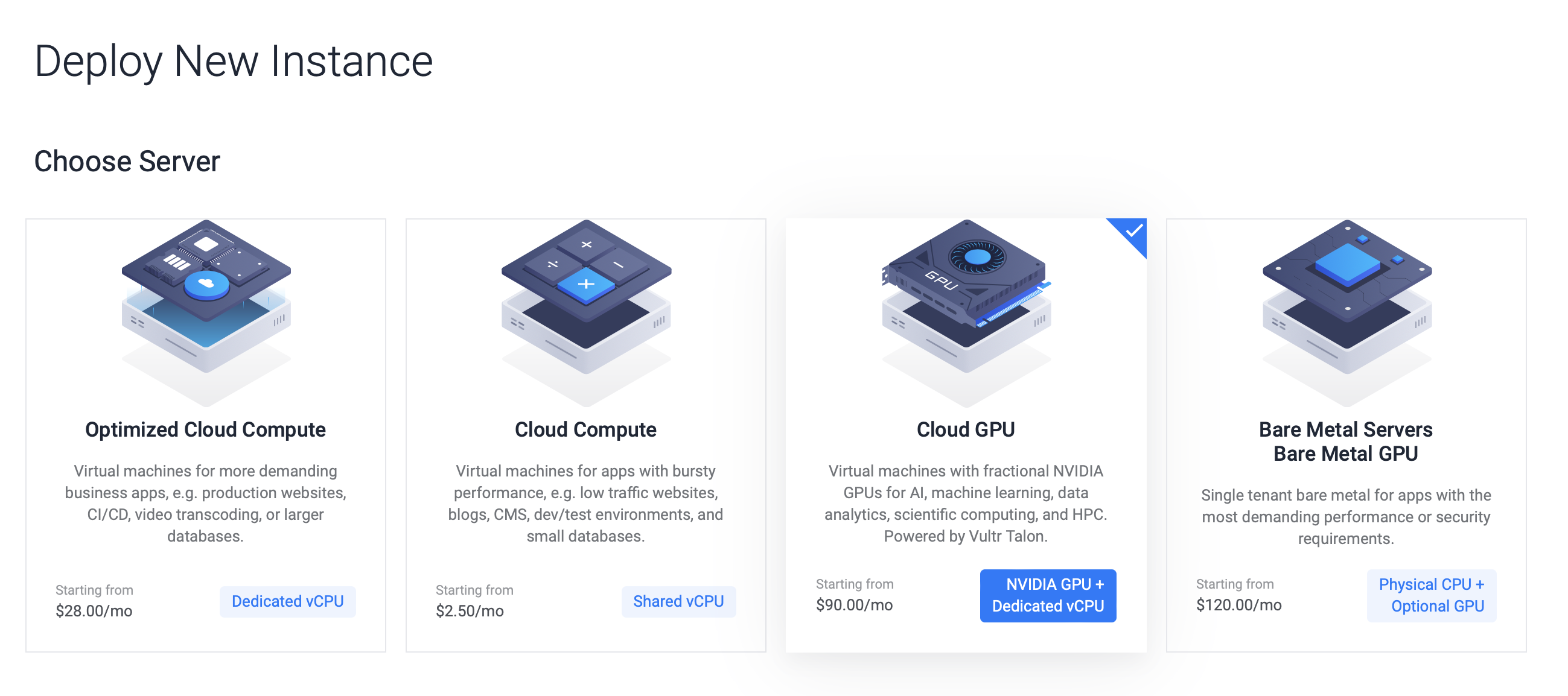
Select Cloud GPU as the server type.

MLDev does not support VPS or Bare Metal instances.
Choose the server GPU.
- NVIDIA A100 - Optimized for AI, data analytics, and HPC workloads.
- NVIDIA A40 - Professional graphics designed for creative and scientific challenges.
Choose the server location.
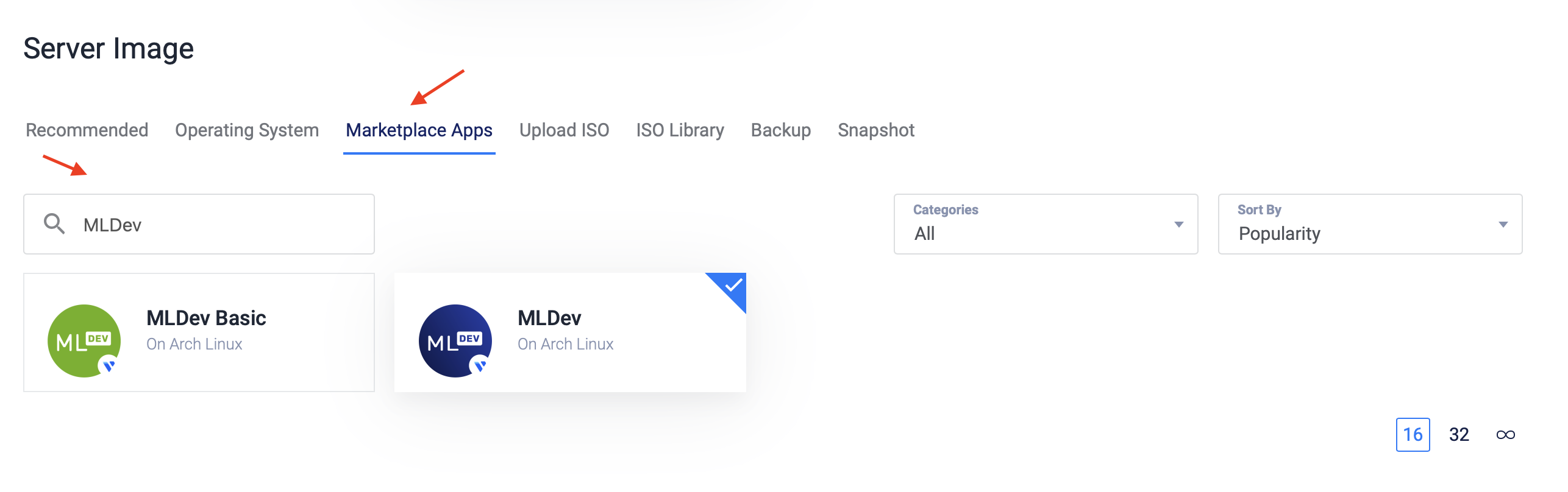
Choose a server image from Marketplace Apps.
Choose the server size.
Choose the server options (Auto Backups, IPv6, DDOS Protection, and so on).
Enter your username in the Marketplace App Requested Information field.
Add SSH keys.
Choose a server hostname and a label to identify it in the customer portal, then click Deploy Now.

The deployment takes several minutes.

Securing the Vultr Cloud Server

The deployed server isn't fully secure by default. Following the security precautions will ensure that the server is not susceptible to potential attacks.

Regular System Updates

Performing regular system updates not only gives you the newest features but is an essential process to make sure that security vulnerabilities don't affect you.

If you're not familiar with updating your server, read the guide on How to Update a Vultr Cloud Server.

Managing Privileges

It is a good practice to use the least amount of privilege when performing tasks on your server. The principle of least privilege is a security concept that involves giving programs and users only the minimum level of access necessary to complete their tasks.

In Unix-like systems, there are differences between root (superuser account) and sudo (superuser do, a command-line utility) regarding privilege escalation.

If you're unfamiliar with the concept, refer to the system-specific guide on How to use Sudo on a Vultr Cloud Server.

Setting up a Vultr Firewall

Allowing inbound and outbound connections from the server can be configured using Vultr Firewall.

For example, you could allow SSH connections just on port 22, or VNC connections on just port 5900.

See a more detailed overview of the Vultr Firewall.

Example Usage

Test out the deployed Cloud GPU with a machine learning project in Python, using SciPy.

Open the terminal and follow the steps.

1. Install Prerequisites

Open your terminal and install scipy, numpy, matplotlib, pandas, and scikit-learn libraries.

Installing the packages via pip:

$ python -m pip install -U scipy numpy matplotlib pandas scikit-learn

Installing the packages via conda:

$ conda install scipy numpy matplotlib pandas sklearn

2. Import Libraries

Import all libraries and tools necessary for the completion of the guide.

Either run the command python, or create a new file for the example using nano ml.py.

from pandas import read_csv
from pandas.plotting import scatter_matrix
from matplotlib import pyplot

3. Load The Data

You are going to use the penguins dataset. This is one of the most common datasets. More datasets can be found in the seaborn-data repository.

The dataset contains 344 penguin characteristics, with different measurements, locations, masses, and so on.

In this step, you're going to load the dataset from a csv file.

url = "https://raw.githubusercontent.com/mwaskom/seaborn-data/master/penguins.csv"
ds = read_csv(url)

4. Data Overview

You're going to overview the data in these ways:

Dataset Dimensions
Data Preview
Statistical Attribute Summary
Data Breakdown

To see how many instances and how many attributes the data contains you can use the shape property.

print(ds.shape)

The penguins dataset should return this:

(344, 7)

To see the first n rows of the data, use the head property. Update the n to the number of rows you'd like to be shown.

n = 10
print(ds.head(n))

The output will show the first n rows:

species     island  bill_length_mm  bill_depth_mm  flipper_length_mm  body_mass_g     sex
0  Adelie  Torgersen            39.1           18.7              181.0       3750.0    MALE
1  Adelie  Torgersen            39.5           17.4              186.0       3800.0  FEMALE
2  Adelie  Torgersen            40.3           18.0              195.0       3250.0  FEMALE
3  Adelie  Torgersen             NaN            NaN                NaN          NaN     NaN
4  Adelie  Torgersen            36.7           19.3              193.0       3450.0  FEMALE
5  Adelie  Torgersen            39.3           20.6              190.0       3650.0    MALE
6  Adelie  Torgersen            38.9           17.8              181.0       3625.0  FEMALE
7  Adelie  Torgersen            39.2           19.6              195.0       4675.0    MALE
8  Adelie  Torgersen            34.1           18.1              193.0       3475.0     NaN
9  Adelie  Torgersen            42.0           20.2              190.0       4250.0     NaN

You can take a look at the attribute summary. Use the describe property:

print(ds.describe())

The summary will provide generic statistical information, like the count, mean, min/max values, and percentiles.

bill_length_mm  bill_depth_mm  flipper_length_mm  body_mass_g
count      342.000000     342.000000         342.000000   342.000000
mean        43.921930      17.151170         200.915205  4201.754386
std          5.459584       1.974793          14.061714   801.954536
min         32.100000      13.100000         172.000000  2700.000000
25%         39.225000      15.600000         190.000000  3550.000000
50%         44.450000      17.300000         197.000000  4050.000000
75%         48.500000      18.700000         213.000000  4750.000000
max         59.600000      21.500000         231.000000  6300.000000

Species (or any other attribute) distribution breakdown is done with groupby property:

print(ds.groupby('species').size())

The species count will be displayed as follows:

species
Adelie       152
Chinstrap     68
Gentoo       124
dtype: int64

5. Data Visualization

Plotting data gives you a better understanding of the data.

You will explore two plot types - univariate and multivariate plots.

A univariate plot, or analysis, looks at only one variable, whereas a multivariate plot looks at more than 2 variables and their relationship.

Perform a univariate plot with the plot property:

ds.plot(kind='box', subplots=True, layout=(2,2), sharex=False, sharey=False)

pyplot.show()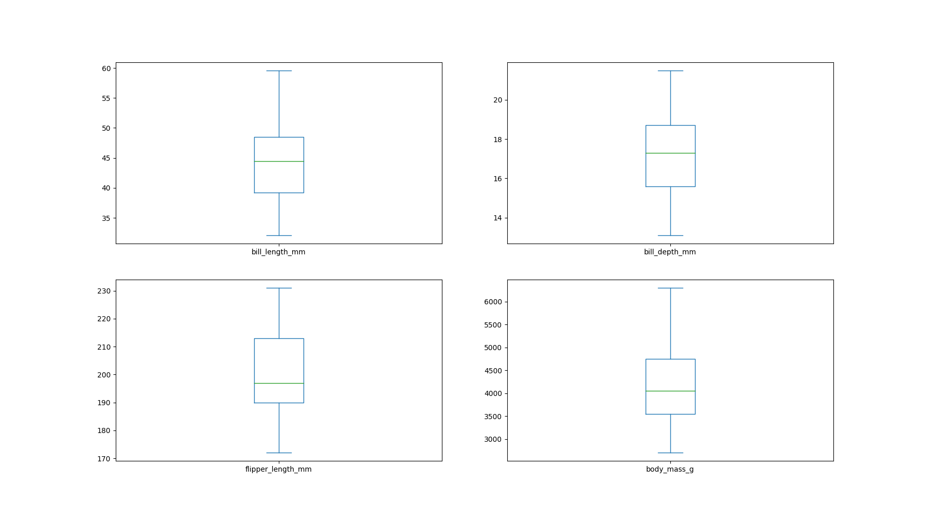

A Univariate Plot

Histograms are also available as a means of data visualization. The hist property will create a histogram of each attribute.

ds.hist()
pyplot.show()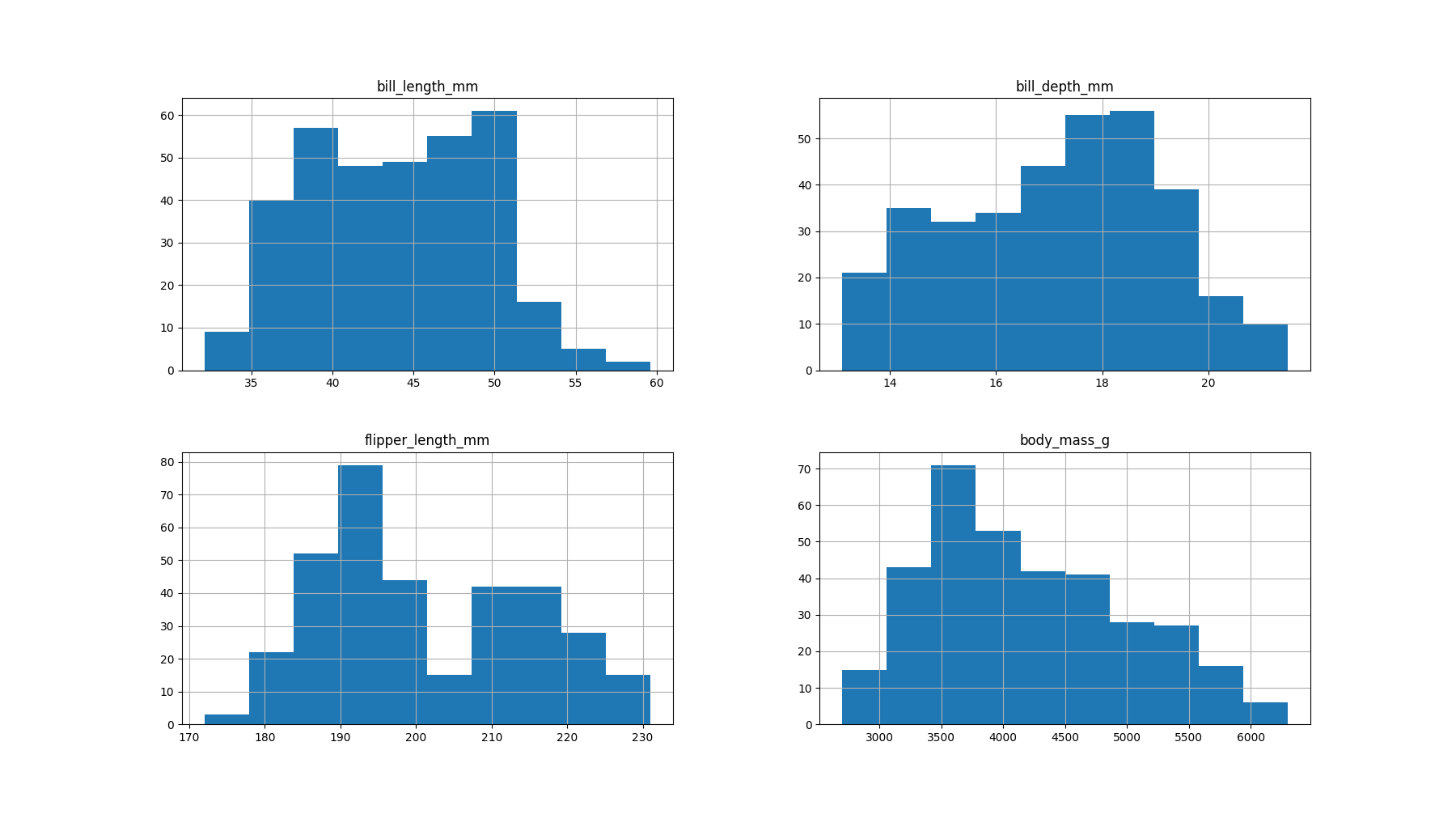

A Histogram

Examine relationship between attributes with multivariate plotting using scatter_matrix().

scatter_matrix(ds)
pyplot.show()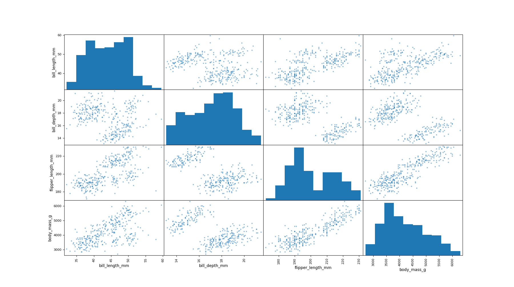

A Multivariate Plot

Next Steps

Python, in combination with adequate modules, can be a powerful tool for machine learning. Expanding this knowledge to be paired with CUDA can help you utilize most of your Cloud GPU resources.

See how machine learning in Python was used to take the First Image of a Black Hole.

Explore the penguin dataset with more mathematical and analytical features with the "penguin dataset: The new Iris" guide.