Explore Foundational Machine Learning Concepts

Introduction

Machine Learning (ML) models are complex algorithms that distributed into multiple types such as linear regression, logistic regression, clustering, neural networks, and so on. Neural network-based models are the basis of modern ML tools such as transformers, diffusers, language models, computer vision models, among others.

This article explains machine learning in the context of artificial neural networks with foundational machine learning concepts grouped into the following parts:

• Definitions and terminology
• Basic principles of Artificial Neural Networks (ANNs)
• Explanation of the training process

Terminologies

Machine Learning includes multiple terminologies. To illustrate a terminology, definitions use the following hypothetical samples such as the following that predicts house prices:

A house-price-prediction model takes information like the built-up area of the house, the number of bedrooms, and the locality as inputs. It uses these factors to predict the price of the house. The model predicts the price of a house and compares it against other known market prices to estimate the model's accuracy.

The above example describes a model you can train using market data about the prices of different houses and properties. After training, the model can be used to:

• Estimate the price of a house whose market price is not yet known.
• Estimate whether a house has a fair market value.

Output Variable

The output variable, or dependent variable represents the task performed using the model. The variable is the quantity the model is expected to predict. In the house prediction example, the output variable is the predicted price of an individual house.

True Value

The real-world value of the output variable for a given input is the true value or actual value. In the example of a house-price prediction model, the market price of a specific house is the true value of the output variable.

Predicted Output

The value of the output variable as computed by the model is the predicted output, also called the predicted value. The predicted output in the earlier example is the price of the house as calculated by the model.

In general, the predicted output is not equal to the true output. A good model makes better predictions than a bad model while the features, parameters, and bias compute the predicted output.

Features

Features are the factors the model uses to make its prediction. They are also called independent variables. In the earlier example, the number of bedrooms, the total built-up area, the locality, and the number of floors are features the model can use to predict the house price.

Feature Engineering

Perform pre-processing of available features before using them in a model is a common practice referred to as feature engineering that covers the following two main aspects:

• The Deciding features to use to make predictions. It's good practice to use only a small number of highly relevant features.
• Transforming input data into more useful forms. For example, normalizing the input data so that all values are within a specific range.

Synthetic Features

A synthetic feature involves combining two or more individual features to make a single more meaningful feature that does not exist in the original data. For example, in a model that predicts housing prices, the length and breadth of the compound of a residential property can be combined to make a synthetic feature such as the total area.

Model Weights (Parameters)

Parameters also known as model weights, denote the relative significance of each feature in predicting the output. Each model has a corresponding feature mathematically combined with the corresponding weights In the example model:

• If the price of a house depends on its locality instead of the number of bedrooms, then the locality factor has a higher weight than the number of bedrooms.

Bias Term

The bias term denotes the baseline value of the output variable. In a linear X-Y graph, the bias is the Y-intercept. The bias is the value of the output variable if the weights of all the features are set to zero. For example, in the house price prediction model:

• The bias can represent the minimum (non-zero) price floor for a house, regardless of any other factors.

Basic Principles of Artificial Neural Networks (ANNs)

Models based on Artificial Neural Networks (ANNs) are used for complex tasks such as Natural Language Processing (NLP), image recognition, and many more. This section explains the key components for building ANNs.

Neurons

ANNs use a grouped sequential layer of neurons to form basic ML building blocks for neural networks. Individually, ANNs perform elementary tasks such as tensor multiplication. Each neuron is parametrized with a tensor of weights with the following tasks:

• Multiply the weight tensor with the input tensor to compute the weighted sum.
• Pass the sum through activation functions.
• Pass the output to the neuron(s) in the next layer.

Below is a rough mathematical representation of how an individual neuron works:

z = w1.x1 + w2.x2 + ... + wn.xn + b  

y = A(z)

Within the representation, the values run as:

• x1, x2: The neuron input features of the neuron.
• w1, w2: Set of Neuron weights.
• b: The Neuron bias term.
• z=: The calculation expression also known as the neuron transfer function
• A is the activation function of the layer.
• y is the neuron's output that forms the input of the neurons in the next layer.

Mathematically, the output, inputs, weights, and biases run as tensors. Thus:

• x can be represented as [x1, x2, ...].
• y can be represented as [y1, y2, ...].
• w can be represented as [w1, w2, ...].

Every neuron in the network implements a similar operation. The goal of the training process is to calibrate the values of the weights and biases such that the model makes accurate predictions.

Artificial Neural Networks

Artificial Neural networks consist of interconnected layers of neurons. Neurons in each layer are interconnected with previous layer and next layer neurons. In a simplistic model, the input data passes sequentially through each layer of neurons. Then, each layer processes the data it receives and passes its output to the next layer. The final layer gives the model's output.

The following PyTorch code snippet defines a sample implementation of the layers in a rudimentary neural network:

import torch
import torch.nn as nn

model = nn.Sequential(
    nn.Linear(4, 16),

    nn.Linear(16, 8),
    nn.ReLU(),

    nn.Linear(8, 1),
    nn.Sigmoid()
)

print(model)

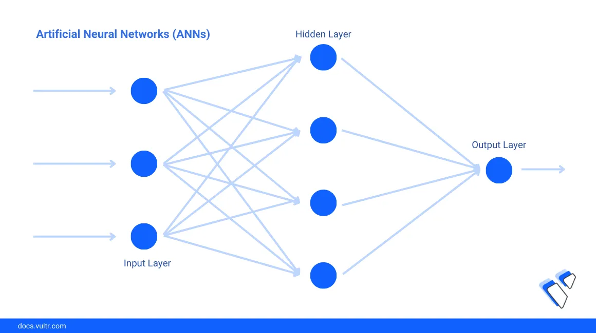
The above network consists of an input layer, one hidden layer, and an output layer explained in the following sections.

Input Layer

The input layer encodes features that are used to model the data and receive the input data. The number of neurons in the input layer corresponds to the number of features in the model. In the example of a real estate model, the input layer consists of one neuron for each feature such as a built-up area and number of bedrooms.

nn.Linear(4, 16),

The above PyTorch code defines an input layer with 4 input neurons and 16 output neurons. Based on the implementation, the input layer then connects to the first hidden layer.

Hidden Layers

One or more hidden layers transform the input in stages. Each stage broadly represents a particular aspect of the data. For example, in a facial recognition model, one of the hidden layers may recognize the color of the eyes. The hidden layers are largely responsible for the model's performance. The number of hidden layers and the number of neurons in each layer depends on the complexity of the model. For example, a large language model should have more layers with more neurons per layer, compared to a real estate pricing model.

nn.Linear(16, 8),
nn.ReLU(),

In the above code, a hidden layer is defined with 16 input neurons and 8 output neurons. Then, the output is fed through the ReLU activation function.

Hidden layers are parametrized as follows:

• Each neuron is associated with a bias term.
• The connection between each pair of neurons is associated with a weight.

Operationally, a hidden layer neuron receives an input value from every neuron it connects to in the previous layer and the last hidden layer connects to the output layer.

Output Layer

The Output layer accepts the result from the last hidden layer and applies another activation function to give the model's output. In the house price prediction model, the output layer can be a single neuron with the predicted house price.

nn.Linear(8, 1),
nn.Sigmoid()

The above code defines an output layer with 8 input neurons and 1 output neuron. The output neuron is fed into a Sigmoid activation function.

For more information on how to define a neural network using PyTorch, visit the PyTorch tutorial on neural networks.

Model predictions depend on the values of the network's weights and biases. The training process determines the values of weights and biases that result in accurate predictions. The following sections explain the concepts used to train machine learning models.

Model Training

Training is the process of using sample data to determine a set of model parameters that make the most accurate predictions. In the hypothetical example about predicting house prices, the training examples consist of market data about the features and market prices of different houses.

The following steps describe the training process:

• The training data which consists of input pairs and corresponding outputs is split into training and validation datasets.
• Models are initialized with a random set of weights and biases. Thus, the model has low accuracy.
• The weights and biases compute the predicted output for different examples in a process called forward pass.
• The difference between the predicted output and the actual output is calculated using the loss function.
• The loss is used to update the values of the model's weights in a process called the backward pass, or backpropagation of errors to update the model parameters.

Each training iteration includes a forward pass followed by backpropagation of the loss. Training iterations continue until it finds a set of values that make accurate predictions. The goal of training is to maximize the model's accuracy.

The following code illustrates an outline of the training algorithm:

# data set definitions for my_dataset

# parameter definitions for n_epochs(number of epochs), learning rate, batch size

data_training, data_validation = torch.utils.data.random_split(my_dataset, [0.8, 0.2])
data_loader_training = torch.utils.data.DataLoader(data_training, batch_size = <batch_size>, shuffle = True)

loss_function = nn.NLLLoss()
optimizer = torch.optim.Adam(params = model.parameters(), lr = <learning_rate>)

for i in range(n_epochs):
    for (index, batch_data_training) in enumerate(data_loader_training):

        # calculate the predicted output - forward pass
        output_predicted = model(batch_data_training)

        # compute the loss
        loss = loss_function (output_predicted, output_true)

        # back propagation
        loss.backward()
        optimizer.step()

How Training Processes Use Data

A trained model performs well on new data samples. Hence, the training process also tests the model's performance on new sample data values. To achieve this, the entire dataset distributed into two subsets and not entirely served to the model during training. The subsets include:

• Training set: A subset of examples is used to train the model.
• Validation set: Consists of the remaining examples used to test the model's performance.

The ratio between the training set and the testing set is called the train-test split. For example, an 80-20 split of the dataset means that 80% of the examples are used in training and 20% for testing the model. The following code snippet below splits the dataset my_dataset with an 80-20 split:

>>> data_training, data_validation = torch.utils.data.random_split(my_dataset, [0.8, 0.2])

Based on the above summary, you can train the model with your own dataset. For more information, learn more about tools for handling data in PyTorch.

Data Batches

For each iteration, the model uses a subset of the training dataset called a batch. The number of examples used for each training iteration create a batch size that depends on:

• The amount of compute resources needed to process each example.
• The amount of available compute resources.

It's a common practice to use a data loader function to distribute a dataset into random batches. Then, the training process iterates through each of the random batches. The following code uses a data loader to create an iterator that consists of the training data:

>>> data_loader_training = torch.utils.data.DataLoader(data_training, batch_size = <batch_size>, shuffle = True)

For more information about data loaders, bisit the PyTorch data tutorial.

When a model covers all examples in the training set, the completion is marked as one epoch. It's common to run training over multiple epochs. The training continues until the model minimizes the average difference between the true value and the predicted value of the output variable across all the training examples. When the value of the parameters no longer changes significantly from one iteration to the next, the model is noted to have converged.

Forward Pass

In a forward pass, the model evaluates training examples. For each example, it computes the model's predicted output and compares it with the true output. The difference between the true output and the predicted output is called the loss. A more accurate prediction has a lower loss value.

The following code is a common way of defining the forward pass of a network:

>>> def forward(self, input):
    output = self.model(input)
    return output

The forward pass is invoked by applying the model on an example data point such as:

>>> output_predicted = model(input)

Backpropagation

In backpropagation, the model's weights and biases are updated depending on the loss computed in the forward pass. This is referred to as backpropagating errors through the network. The function which updates the model parameters is called the optimizer. After updating the model parameters, it runs another forward pass to process the next set of training examples using the updated model parameters. Thus, it re-computes the loss for the new set of parameters and the iterations continue until the model is trained.

Backpropagation is commonly invoked with the following functions:

>>> loss_function.backward()
>>> optimizer.step()

Activation Functions

An activation function:

• Decides whether the output of a particular neuron should be considered or ignored.
• Converts the output of a neuron into the input of the next neuron.
• Introduces non-linearity into the neural network. Operations performed by a neuron are based on linear algebra. So, the input undergoes a linear transformation into the output. However, real-life tasks tend to follow non-linear patterns. Hence, it's necessary to introduce non-linearity into the neural network.

There are many activation functions. The choice of activation depends on the network architecture, the nature of the data, and the task at hand. To explore different activation functions, visit the PyTorch documentation on neural networks.

The following sections explain the commonly used activation functions.

Sigmoid Function

The sigmoid function, also known as the logistic function, maps any real-valued input to a number between 0 and 1. Graphically, it is an S-shaped curve.

It's commonly used in:

• Binary classification problems: If the separation boundary between the two classes is not a straight line. In such cases, a non-linear function is needed to model the decision boundary.
• The output layer of a neural network: If the goal is to map the network's output to a probability between 0 and 1.

The Sigmoid function is invoked using the following function in PyTorch.

>>> nn.Sigmoid()

For more information about the Sigmoid function, visit the package's PyTorch documentation.

ReLU

Rectified Linear Unit (ReLU) is a piecewise linear function. The default function value is zero for negative values of the input and equal to the input for positive values. Over the entire range, it's a non-linear function that represents complex data relationships. As a result, ReLU is a preferred activation function for the hidden layer of deep learning networks

The following code invokes ReLU in a model environment:

>>> nn.ReLU()

For more information, visit the PyTorch documentation on the ReLU function.

Softmax function

The Softmax function is used when the output should consider all elements in the input vector and works with the following 2 stages:

• The first step: Maps an input vector into a vector of ratios. The output of each input vector element is the ratio of the exponential of that element to the sum of the exponentials of all the elements in the input vector.
• The second step: The Softmax function selects the element with the highest ratio output.

You can apply the Softmax function with:

• Multiclass classification problems.
• The output layer of neural networks.

Use the following code to invoke the Softmax function in PyTorch:

>>> nn.Softmax(dim= <dimensions>)

For more information, visit the Softmax function PyTorch documentation.

Loss

Loss is the difference between the model's predicted output and the true output. A good prediction has a lower loss than a bad prediction. A loss mathematical function expresses the loss by estimating the accuracy of the model during the training and evaluation of ML models. Mathematically, the goal of training a model is to find a set of weights and biases that reduce the loss function.

The loss is calculated by passing the true output and the predicted output to the loss function similar to the following example:

>>> loss = loss_function(output_predicted, output_true)

Experiment with different loss functions to find out which works best for a given dataset and problem. For example, with the following two common loss functions.

Mean Squared Error (MSE)

MSE (Mean Squared Error) is the square of the difference between the true output and the predicted output. The following code defines a loss function that uses the MSE loss.

>>> loss_function = nn.MSELoss()

For more information about the loss function, visit the MSE PyTorch documentation.

Log Loss

Log loss is based on cross-entropy which represents the difference between two probability distributions. For logistic regression, the two probability distributions include the true output and the predicted output. It's used in classification-based problems and the following code snippet defines how to set a loss function that uses a Log loss:

>>> loss_function = nn.NLLLoss()

For more information, visit the PyTorch documentation on the Log Loss function.

Optimizer

The optimizer updates model parameters during the training process with the following functionalities:

• Generates a limited set of potential updates to the parameter values because it's impossible to randomly try all possible values for the model parameters.
• Evaluates the most suitable set of values to update the model parameters.
• Updates the parameters in each iteration.

To decide the amount by which to update the model's parameters, the optimization algorithm uses the gradient of the loss function and the learning rate as explained in the following sections.

Gradient

The gradient represents the change in the value of the loss in the model's parameters. Thus, it represents the rate of change of the loss in relation to the model weights. Mathematically, the gradient is expressed as the partial derivative of the loss function in relation to all the model parameters.

When the loss function is at its minimal value, its gradient is theoretically zero. Machine learning libraries such as PyTorch have pre-built functions that calculate the gradient using numerical computation techniques. A gradient is calculated with the following function:

>>> loss_function.backward()

For more information, visit the PyTorch documentation on gradients.

Common Optimizers

Different optimizers take different approaches to perform the same task of updating the model's parameters iteratively. The choice of an optimizer depends on the task at hand. The optimizer is typically invoked as below:

>>> optimizer.step()

For more information about optimizers, visit the PyTorch documentation on optimization. The following sections discuss two of the commonly used optimizers.

Gradient Descent

In Gradient Descent, the amount by which each weight is updated in each training iteration is the product of:

• The gradient (partial derivative) of the loss function in relation to the weight.

• The learning rate which is manually set to a constant value.

  The following code instantiates the Gradient Descent optimizer in PyTorch:

  python Copy

  >>> optimizer = torch.optim.SGD(params = model.parameters(), lr = <learning_rate>)
  

Gradient descent iterations can be achieved in the following ways:

• Batch gradient descent: For each iteration, this algorithm calculates the total gradient of the batch as the sum of the gradients of each data point. The model parameters are adjusted proportionally to this total gradient. This method is suitable for smaller datasets that fit in memory at once. To use Batch gradient descent, use the data loader to choose a batch size equal to the size of the training dataset.

• Stochastic gradient descent: In each iteration, the algorithm updates the model parameters based on the gradient of each data point in the training set. This method is suitable for large datasets the model can't process at the same time. Because it processes only one item at a time, it uses less memory and results in faster updates. To use Stochastic gradient descent, use the data loader to choose a batch size equal to 1.

For more information, visit the Stochastic Gradient Descent PyTorch documentation. To implement optimization concepts, it's important to test with modern optimizers such as Adam that are based on the gradient descent.

Adam Optimizer

Adaptive Moment Estimation (Adam) is a common optimizer and the default choice in many modern ML models. The main working principles of this optimizer include:

• Modifying the learning rate depending on the gradient. Weights with larger gradients have a lower learning rate, and vice versa.

• Consideration of the present and previous steps gradient. Gradients are exponentially weighted and added up to compute the function moving average.

• Assigning higher weights to gradients from recent iterations than to those from older iterations.

  In PyTorch, the Adam optimizer is instantiated using the following function.

  python Copy

  >>> optimizer = torch.optim.Adam(params = model.parameters(), lr = <learning_rate>)
  

For more information, visit Adam PyTorch documentation.

Conclusion

You have explored important machine learning concepts with a brief overview of the training process and functions used to train modern models. These principles are important when using different ML models and work as a background for more advanced deep learning topics.