
How to Deploy a Deep Learning Model with Streamlit

Introduction
Machine learning (ML) and data science are the fastest-growing technology areas. However, machine learning engineers need faster ways to expose their models as web applications without knowledge of web backend or frontend technologies such as Flask, React, and Javascript.
This process is also very time-consuming, more so if the goal is to deploy the model on the web as a prototype. For such scenarios, Streamlit is a perfect solution that can be easily scaled if the load on the application increases.
Streamlit is a free, open-source framework to quickly build and share interactive machine learning and data science web apps. It is a Python-based library specifically designed for data scientists and machine learning engineers.
In the following tutorial, you will train a deep learning model on an image dataset as a multi-classification problem. Although our code is designed to work on both CPU and GPU instances, it is recommended that you use a GPU instance to save time and increase accuracy. After evaluating the prediction metric for the trained model, you will deploy the model in production as a web application using Streamlit and tmux.
Prerequisites
Before you begin this tutorial, you need the following:
A Vultr server with a freshly installed Ubuntu (22.04) instance, preferably a GPU instance.
A local Mac, Windows (with Putty installed), or a Linux system. This guide focuses on Windows, but the procedures are similar for any Linux control node.
A previously generated private SSH Key for the Vultr host; the SSH public key should already be installed for the root user.
A text editor that supports Python syntax highlighting, such as Atom, Visual Studio Code, or Sublime Text. These editors are available on Windows, macOS, and Linux.
Familiarity with Python programming and pip
Familiarity with Machine Learning concepts such as training, testing, evaluation
Familiarity with data science tools such as Numpy, Pandas, Sci-kit-learn, Kera, and TensorFlow.
Connect with SSH
Connect to your freshly installed Vultr server with your private SSH keys as a non-root user.
Also note that by default, you will connect with the Vultr instance terminal shell, which does not show the host and current directory you are in, and does not have an autocompletion feature. Type bash on the terminal if you are used to working with Bash shell:
$ bashInstall the Required Libraries
Machine learning tasks involve using various Python libraries (non-standard), which are most common in data science. To install the required libraries to follow this tutorial:
$ python3 -m pip install streamlit pandas numpy sklearn scikit-learn tensorflowAlso, install the recursive directory listing program tree:
$ sudo apt-get install treeMake Sure the GPU is Available
In this guide, you will be training your model on an image dataset, and therefore it is advantageous to use a vultr GPU instance instead of a normal CPU instance which can accelerate the training phase substantially. This is known as GPU acceleration. Vultr uses Nvidia GPUs (from NVIDIA A100 and A100 series), and it provides computing GPUs at a very cost-effective price which are not shared with other customers.
To check the availability of GPU on the remote machine, launch a python session:
$ python3And type the following in the python session:
>>>import tensorflow as tf
>>>print("Num of GPUs Available: ", len(tf.config.list_physical_devices('GPU')))
You will receive an output that indicates GPUs are available:
[secondary_label Output]
Num of GPUs Available:  1
If your server is not equipped with GPU, Num GPUs Available will be 0.
Leave the Python interpreter by typing Ctrl+D.
Comparative Performance evaluation of GPU versus CPU
In this step, we will ensure that our GPU device is available, and we will make a comparative performance analysis of the GPU versus the CPU.
Create a project folder named satellite and enter into it:
$ mkdir satellite ; cd satelliteWhen in your project folder, create a new file called comparison.py:
$ vim comparison.pyAdd the following lines of python code to the comparison.py file:
import tensorflow as tf
import timeit

device_name = tf.test.gpu_device_name()
if device_name != '/device:GPU:0':
  print(
      '\n\nThis error most likely means that this notebook is not'
      'configured to use a GPU. Change this in Notebook Settings via the'
      'command palette (cmd/ctrl-shift-P) or the Edit menu.\n\n')
  raise SystemError('GPU device not found')

def cpu():
  with tf.device('/cpu:0'):
    random_image_cpu = tf.random.normal((100, 100, 100, 3))
    net_cpu = tf.keras.layers.Conv2D(32, 7)(random_image_cpu)
    return tf.math.reduce_sum(net_cpu)

def gpu():
  with tf.device('/device:GPU:0'):
    random_image_gpu = tf.random.normal((100, 100, 100, 3))
    net_gpu = tf.keras.layers.Conv2D(32, 7)(random_image_gpu)
    return tf.math.reduce_sum(net_gpu)

# We run each op once to warm up; see: https://stackoverflow.com/a/45067900
cpu()
gpu()

# Run the op several times.
print('Time (s) to convolve 32x7x7x3 filter over random 100x100x100x3 images '
      '(batch x height x width x channel). Sum of ten runs.')
print('CPU (s):')
cpu_time = timeit.timeit('cpu()', number=10, setup="from __main__ import cpu")
print(cpu_time)
print('GPU (s):')
gpu_time = timeit.timeit('gpu()', number=10, setup="from __main__ import gpu")
print(gpu_time)
print('GPU speedup over CPU: {}x'.format(int(cpu_time/gpu_time)))
Save your comparison.py file, then run the code in a terminal session:
$ python3 comparison.pyIf your machine has a GPU device, you will receive an output response similar to this:
Time (s) to convolve 32x7x7x3 filter over random 100x100x100x3 images (batch x height x width x channel). Sum of ten runs.
CPU (s):
2.9536721409999984
GPU (s):
0.04097409399997787
GPU speedup over CPU: 72x
Otherwise, you will get an error (if GPU is not there on your machine).
Your speedup may be different depending on your GPU capability. So it is a clear indication that GPUs are highly advantageous if machine learning task involves heavy number crunching, such as in image processing (which the current guide deals with) or natural language processing (NLP).
Now for the current guide, you will train a machine-learning model using image datasets from Kaggle. This dataset has four different classes mixed from Sensors and Google map snapshots. The trained model can recognize a satellite image belonging to a particular class of the four classes. Instead of downloading the data to your local machine, you will download the Kaggle image dataset directly to your server. This trick will be handy when you process a big Kaggle dataset that can run from ~100 MBs to a few GBs.
Download the Kaggle Dataset
For this step, you need an account on Kaggle, as you will need the Kaggle API token. Create a Kaggle account if you don't have one already. To download the Kaggle API token, go to your profile on the Kaggle website from your browser, click on the Account tab, and in the menu ribbon, go to the Account tab as shown below:
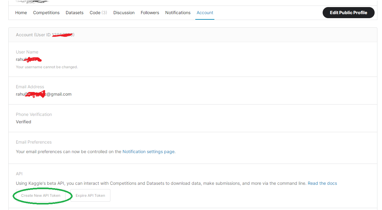
Click on the Create New API Token button. This will download a kaggle.json file to your local machine. Open the JSON file via any text editor on your local machine to view its content which will be similar to:
{"username": "rahulXXXX", "key": "c79b8c0b4e6df5491ed1c3ce9aXXXXXXXX"}Note the values for the username and key keys.
Now create a kaggle_json.py file in the project folder satellite:
$ vim kaggle_json.pyAnd add the following code to it
import os

os.system('mkdir ~/.kaggle')
os.system('touch ~/.kaggle/kaggle.json')

api_token = {"username": "rahulXXXX", "key": "c79b8c0b4e6df5491ed1c3ce9aXXXXXXXX"}

import json

with open('/root/.kaggle/kaggle.json', 'w') as file:
    json.dump(api_token, file)

os.system('chmod 600 ~/.kaggle/kaggle.json')
Modify the username and key values as previously noted from your downloaded kaggle.json file in the above code.
Run the python script:
$ python3 kaggle_json.pyThis python script will create a kaggle.json file on your remote server and grant it the necessary permission.
To download Kaggle datasets, you need to install the Kaggle CLI tool:
$ python3 -m pip install kaggleRun the following command to download your required Kaggle dataset:
kaggle datasets download -d mahmoudreda55/satellite-image-classificationThis command downloads the image data as a zip file from the Kaggle website.
Downloading satellite-image-classification.zip to /content
 87% 19.0M/21.8M [00:01<00:00, 22.4MB/s]
100% 21.8M/21.8M [00:01<00:00, 18.4MB/s]
Unzip the downloaded zip file:
$ unzip satellite-image-classification.zipThis will unzip the image data to a newly created data folder. Check the content of the data folder.
$ ls dataYou will see four folders:
cloudy desert green_area waterThese folders correspond to the four classes of images.
You can check the contents of the folder with tree command:
$ tree data -L 2You will notice that these four directories contain 5631 jpeg images. Also, download the few images from the Kaggle website to your local machine to upload once you run your Streamlit application in the later steps of this tutorial.
Clear the terminal screen.
$ clearNow you will prepare the image for machine learning.
Prepare the Dataset for the Training
Now create a dataPreparation.py file:
$ vim dataPreparation.pyAnd add the following code to this file:
import pandas as pd
import os

# Create an empty dataframe
data = pd.DataFrame(columns=['image_path', 'label'])

# Define the labels/classes
labels = {'data/cloudy': 'Cloudy',
          'data/desert': 'Desert',
          'data/green_area' : 'Green_Area',
          'data/water': 'Water'
           }

# Loop over the train, test, and val folders and extract the image path and label
for folder in labels:
    for image_name in os.listdir(folder):
        image_path = os.path.join(folder, image_name)
        label = labels[folder]
        data = data.append({'image_path': image_path, 'label': label}, ignore_index=True)

# Save the data to a CSV file
data.to_csv('image_dataset.csv', index=False)


import pandas as pd
import numpy as np
from sklearn.model_selection import train_test_split
from keras.preprocessing.image import ImageDataGenerator


# Set batch size based on if CPU only server or server with GPU
import tensorflow as tf

device_name = tf.test.gpu_device_name()
if device_name =='/device:GPU:0':
    batch_size = 32
else:
    batch_size = 8


# read the data in a Panda dataframe

df = pd.read_csv("image_dataset.csv")

# Split the dataset into training and testing sets
train_df, test_df = train_test_split(df, test_size=0.2, random_state=42)
# Pre-process the data
train_datagen = ImageDataGenerator(rescale=1./255,
                                   shear_range=0.2,
                                   zoom_range=0.2,
                                   horizontal_flip=True,
                                   rotation_range=45,
                                   vertical_flip=True,
                                   fill_mode='nearest')


test_datagen = ImageDataGenerator(rescale=1./255)

train_generator = train_datagen.flow_from_dataframe(dataframe=train_df,
                                                    x_col="image_path",
                                                    y_col= "label",
                                                    target_size=(255, 255),
                                                    batch_size=batch_size,
                                                    class_mode= "categorical")

test_generator = test_datagen.flow_from_dataframe(dataframe=test_df,
                                                  x_col="image_path",
                                                  y_col= "label",
                                                  target_size=(255, 255),
                                                  batch_size=batch_size,
                                                  class_mode= "categorical")
In this python script, you create an empty Pandas dataframe data, and define a python dictionary labels with keys as the path information of folders containing images, and corresponding values as strings in line with folders' names. Then you run a for-loop to populate the dataframe data. Then you save this data to a CSV file image_dataset.csv. In the next step, you read the CSV file to a Pandas dataframe df. Then, you divide the images dataset into train and test sets in the 80 by 20 ratio respectively. As an important preprocessing step, you numericise the image pixels because machine learning frameworks can only process numerical arrays. For this purpose, you employ ImageDataGenerator class imported from keras.preprocessing.image, and create train_datagen and test_datagen object instances from this class with suitable parameter values. During the training, machine learning frameworks typically process the data objects in batches. You set the batch size depending on the type of server, whether CPU or GPU. Finally, you invoke a method flow_from_dataframe of the object with the value of parameter dataframe equal to train_df, and assign this object to the variable train_generator. Similarly, test_generator is created with test_df.
Now, let us run the python script:
$ python3 dataPreparation.pyYou will get the output similar to as below:
Found 4504 validated image filenames belonging to 4 classes.
Found 1127 validated image filenames belonging to 4 classes.
After preprocessing the dataset, dividing them into training and testing sets, and saving them into variables, we move on to the next step of setting up your machine learning model.
Set Up the Model
In this step, we will build our deep learning model. Create a modelBuild.py file:
$ vim modelBuild.pyAnd add the following code to it:
# Import libraries
import pandas as pd
import numpy as np
from sklearn.model_selection import train_test_split
from dataPreparation import train_generator, test_generator

from keras.models import Sequential
from keras.layers import Conv2D, MaxPooling2D, Flatten, Dense, Dropout

# Build a deep learning model
model = Sequential()
model.add(Conv2D(32, (3, 3), input_shape=(255, 255, 3), activation='relu'))
model.add(Conv2D(32, (3, 3), activation='relu', input_shape=(64, 64, 3)))
model.add(MaxPooling2D(2, 2))
model.add(Conv2D(64, (3, 3), activation='relu'))
model.add(MaxPooling2D(2, 2))
model.add(Conv2D(128, (3, 3), activation='relu'))
model.add(MaxPooling2D(2, 2))
model.add(Flatten())
model.add(Dense(128, activation='relu'))
model.add(Dropout(0.5))
model.add(Dense(4, activation='softmax'))

model.compile(optimizer='adam', loss='categorical_crossentropy', metrics=['accuracy'])
Here, for your model, you use convolutional neural network (CNN) using Sequential class from keras.models. The code above will build model with 4 CNN layers, with the final layer activated with softmax for multi-output classification. In the last step, you compile the model with the appropriate optimizer, loss, and metric parameters, as well.
Train the Model
Now create a file trainModel.py:
$ vim trainModel.pyAdd the following code to the trainModel.py file:
from modelBuild import model
import tensorflow as tf
import dataPreparation as dP
device_name = tf.test.gpu_device_name()
if device_name =='/device:GPU:0':
    epochs = 20
else:
    epochs = 1

history = model.fit_generator(dP.train_generator, epochs=epochs, validation_data=dP.test_generator)

model.save('Model.h5')
To train the model for predetermined iterations, you need to set the value of epoch parameter depending upon the availability of GPU on your server; it is set to 20 for the GPU server and 1 for the server with CPU only. For the determined epochs, you train the model by invoking the fit_generator method of the CNN model, and the progress of the training is saved in the history variable for future analysis of how the training proceeded. In the end, you save the trained model as Model.h5 file.
Run the script:
python3 trainModel.pyAlthough the code has been designed and tested to run on the single CPU-only server as well, if the RAM and other computing resources do not match up, you may encounter the Resource Exhausted error as well:
2023-02-06 22:25:13.517504: W tensorflow/core/framework/op_kernel.cc:1830] OP_REQUIRES failed at mkl_util.h:771 : RESOURCE_EXHAUSTED: OOM when allocating tensor with shape[7620608] and type uint8 on /job:localhost/replica:0/task:0/device:CPU:0 by allocator mklcpuIf you face this error, try reducing the batch size from 8 to 4 or 2, and run the training script again. Alternatively, you can launch a GPU instance.
If the training is successfully completed, you will see similar output:
<ipython-input-22-89e63a39d5f5>:1: UserWarning: `Model.fit_generator` is deprecated and will be removed in a future version. Please use `Model.fit`, which supports generators.
  history = model.fit_generator(train_generator, epochs=1, validation_data=test_generator)
141/141 [==============================] - 90s 635ms/step - loss: 0.5479 - accuracy: 0.7023 - val_loss: 0.4773 - val_accuracy: 0.7489
Typically the training time will vary between 5 to 20 minutes with GPU for 20 epochs of training. You can do an experiment with epoch numbers yourself and reach the optimal number by trial and error.
Evaluate the Model
In this step, you will make an inference using the trained model. For that, create a file prediction.py
$ vim prediction.pyAnd add the following code to it:
from tensorflow.keras.models import load_model

import numpy as np
from tensorflow.keras.preprocessing.image import load_img, img_to_array

# Load the model
model = load_model("Model.h5")

# Define the class names
class_names = ['Cloudy', 'Desert', 'Green_Area', 'Water']

# Load an image from the test set
img = load_img("data/green_area/Forest_1768.jpg", target_size=(255, 255))

# Convert the image to an array
img_array = img_to_array(img)
print(img_array)

print(img_array.shape)

img_array = np.reshape(img_array, (1, 255, 255, 3))

# Get the model predictions
predictions = model.predict(img_array)
print("predictions:", predictions)

# Get the class index with the highest predicted probability
class_index = np.argmax(predictions[0])

# Get the predicted class label
predicted_label = class_names[class_index]

print("The image is predicted to be '{}'.".format(predicted_label))
In the code above, you input an image from the green_area folder to the trained model to infer the label. The image is converted to a numerical array and reshaped before inputting it into the trained model. During the training phase, the conversion to numerical array and reshaping was done by ImageDataGenerator implicitly.
Run the python script:
$ python3 `prediction.py`If the code runs successfully, you will see a similar output at the bottom:
1/1 [==============================] - 0s 300ms/step
predictions: [[0.00000e+00 0.00000e+00 1.00000e+00 6.09927e-10]]
The image is predicted to be 'Green_Area'.
In this instance, the model inferred correctly. However, your image prediction may be different depending on the accuracy of your trained model and the image you provide.
Open the Firewall Ports
Before we code the Streamlit application, it is to be noted that by default, on a freshly installed Vultr server, the standard Linux firewall blocks ports for security reasons. Therefore, you will open the required port. Streamlit uses port numbers starting from 8501 onwards. Now to check the firewall status, type in the terminal:
$ sudo ufw status verboseYou will observe a similar response:
Status: active
Logging: on (low)
Default: deny (incoming), allow (outgoing), disabled (routed)
New profiles: skip

To                         Action      From
--                         ------      ----
22/tcp                     ALLOW IN    Anywhere
22/tcp (v6)                ALLOW IN    Anywhere (v6)
Now open port 8501 to listen to the incoming requests:
sudo ufw allow 8501Ensure that port 8501 is open now by checking the status:
sudo ufw status verboseYou will get the output:
Status: active
Logging: on (low)
Default: deny (incoming), allow (outgoing), disabled (routed)
New profiles: skip

To                         Action      From
--                         ------      ----
22/tcp                     ALLOW IN    Anywhere
8501                       ALLOW IN    Anywhere
22/tcp (v6)                ALLOW IN    Anywhere (v6)
8501 (v6)                  ALLOW IN    Anywhere (v6)
So you can confirm that port 8501 is open, and can listen to HTTP requests from any network (IP address). You should open other ports in line 8500 if needed.
Note: Streamlit does not give any warning even if port 8501 is closed. So be sure about the port used by Streamlit is open before you deploy the Streamlit application.
Deploy the Model with Streamlit
In this step, you will deploy your trained model as a web application using Streamlit. It will generate all the necessary endpoints on the back-end server and necessary client-side code (HTML and javascript) to be rendered by the browser. Moreover, the application generated will be responsive, i.e., it will work perfectly on mobile as well as desktop screens.
The web application will upload the test image on the browser by the front-end code. The image will be sent back to the server, and the model will make an inference and send back the inferred result to the front-end.
Create a file main.py:
$ vim main.pyAnd add the following code to it:
import streamlit as st

from tensorflow.keras.models import load_model

import numpy as np
from tensorflow.keras.preprocessing.image import load_img, img_to_array
from PIL import Image

st.header("Image Recognition App")
st.caption("Upload an image. ")
st.caption("The application will infer the one label out of 4 labels: 'Cloudy', 'Desert', 'Green_Area', 'Water'.")
st.caption("Warning: Do not click Recognize button before uploading image. It will result in error.")

# Load the model
model = load_model("Model.h5")

# Define the class names
class_names = ['Cloudy', 'Desert', 'Green_Area', 'Water']


# Fxn
@st.cache
def load_image(image_file):
        img = Image.open(image_file)
        return img

imgpath = st.file_uploader("Choose a file", type =['png', 'jpeg', 'jpg'])
if imgpath is not None:
    img = load_image(imgpath )
    st.image(img, width=250)

def predict_label(image2):
    imgLoaded = load_img(image2, target_size=(255, 255))
    # Convert the image to an array
    img_array = img_to_array(imgLoaded)    #print(img_array)

    #print(img_array.shape)

    img_array = np.reshape(img_array, (1, 255, 255, 3))

    # Get the model predictions
    predictions = model.predict(img_array)
    #print("predictions:", predictions)

    # Get the class index with the highest predicted probability
    class_index = np.argmax(predictions[0])

    # Get the predicted class label
    predicted_label = class_names[class_index]
    return predicted_label
if st.button('Recognise'):
    predicted_label = predict_label(imgpath)
    st.write("The image is predicted to be '{}'.".format(predicted_label))
Here we have turned the previous code from prediction.py into a function predict_label. And button and write method of streamlit is used to create the input and output widget.
Now run the python script through Streamlit:
$ streamlit run main.pyYou will see the following output:
Collecting usage statistics. To deactivate, set browser.gatherUsageStats to False.


  You can now view your Streamlit app in your browser.

  Network URL: http://139.84.xxx.xxx:8501
  External URL: http://139.84.xxx.xxx:8501
Go to your browser and type in the External URL to view your Streamlit application. Depending on the settings of your server, Network URL External URL might be different as well. The screenshot of the app is here.
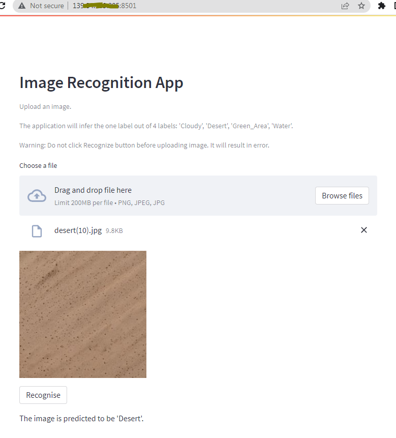
You can play with it by uploading an image out of the previously saved images from the Kaggle dataset on your local machine.
This is all good, but as soon as you close the SSH terminal window or log off, the process will stop, causing your application to stop as well. To overcome this problem, you need to launch the process as a background application.
Stop your application by typing Ctrl+:key_c.
Add Persistentence with Tmux
Tmux is a terminal multiplexer, and Tmux sessions are persistent, which means that programs running in Tmux session will continue to run even if you get disconnected from the terminal. Tmux is already installed in Vultr server(ubuntu image). In case tmux is not installed, install it by:
$ sudo apt-install tmuxStart a new Tmux session with a session name, say sts:
$ tmux new -s stsSee the session name at the left bottom of the console window in a green highlighted info line at the bottom of the terminal window. Start running the Streamlit application in the tmux session:
$ streamlit run main.pyYou will be able to view your application at the External URL as in the previous step. Now detach your Tmux session so that it continues running in the background even when you leave the SSH shell. Now to detach your TMUX session, press Ctrl+B and then D (Don't press Ctrl while pressing D). Be careful not to press Ctrl+C while detaching.
After detaching, you will come back to the SSH console, indicated by no green highlighted line at the bottom. You can now safely close your SSH session, but the application will keep running at the External URL.
Remember if you want to stop the Streamlit application running via a Tmux session, you need to kill the process as follows.
Watch all the Tmux sessions running:
$ tmux lsAttach to the session in which you have started the Streamlit application:
$ tmux attach -t stsWhile in Tmux session, press Ctrl+C to stop the application and then detach by pressing Ctrl+B and then D. Mind it, as the previous step will stop the application.
Note: If you enter into the Tmux session as a root user, you will land in the home folder of root even if you were in your project folder before. Enter into the project folder before running the Streamlit command.
Conclusion
In this tutorial, you trained a machine learning model with image recognition capability, which you subsequently deployed using Streamlit and Tmux. As part of the next actions, you can train machine learning models for NLP and business datasets apart from other image datasets. For inputs to these models, you will use the other input widgets of Streamlit, such as textbox, radio button, and slider. Further as an exercise, you can try to code logic to take care of the error arising in this application if you press Recognise button without first uploading a photo.
More Information
- If your dataset is big, you can use more resource-rich Vultr GPUs.
- If your machine learning framework is pyTorch, you can use Torchserve as well instead of Streamlit.
- For facial recognition, use Vultr GPUs