AI Image Manipulation with Stable Diffusion ControlNet on Vultr Cloud GPU

Introduction

ControlNet is a neural network structure used in diffusion models to control final image generation through various techniques such as pose, edge detection, and depth maps. It provides an efficient way for an AI model to detect which parts of an input image require changes. Thus, it enables Stable Diffusion models to use additional input before manipulating the image and generating a more desired output.

This article describes ways you can perform image manipulation with Stable Diffusion ControlNet on a Vultr Cloud GPU server. You are to manipulate images using ControlNet methods that generate different results based on unique prompts.

Prerequisites

• Deploy a Ubuntu A100 Cloud GPU server with at least:

  • 1/3GPU
  • 20 GB VRAM
  • 3 vCPUs
  • 30 GB Memory

• Use SSH to access the server as a non-root user with sudo privileges

• Switch to the non-root sudo user account

    # su user-example

ControlNet Methods

Below are the Image manipulation ControlNet methods applied in this article:

• Canny Edge Detection
• Depth Map
• Multiscale Line Segment Detector (M-LSD) Detection
• Normal Map
• Pose Detection
• Image Segmentation

Set Up the Server

To run ControlNet models on the server, install the necessary Python dependency packages and set up Jupyter Notebook to run the model in a graphical environment session as described in the following steps.

1. Install PyTorch

    $ pip3 install torch torchvision --index-url https://download.pytorch.org/whl/cu118

   The above command installs PyTorch with the pre-built CUDA 11.8 libraries. To download the latest version, visit the PyTorch Documentation

2. Install Jupyter Notebook

    $ pip3 install notebook

3. Allow the default Jupyter Notebook port 8888 through the firewall to accept incoming connections

    $ sudo ufw allow 8888/tcp

4. Restart the firewall to update the changes.

    $ sudo ufw reload

5. Launch Jupyter Notebook.

    $ jupyter notebook --ip=0.0.0.0 

   The above command starts Jupyter Notebook and accepts connections from all addresses as declared by the --ip=0.0.0.0 option. In case the command fails to run, quit your SSH session and re-establish a connection to your server to activate the Jupyter library.

6. In a new web browser session, access the Jupyter Notebook interface using your generated token.

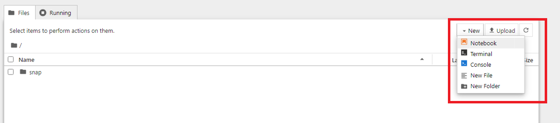
    http://SERVER_IP:8888/tree?token=GENERATED-TOKEN

7. Within the Jupyter Notebook interface, click New, and select Notebook from the dropdown list

   

Install Required Libraries

In this section, install the required ControlNet model libraries used by each method in your Jupyter Notebook file. To run each of the commands described below, press Ctrl + Enter on your keyboard, or click the run button on the main taskbar.

1. Update Jupyter and Ipywidgets

    !pip3 install --upgrade jupyter ipywidgets

2. Install the libraries

    !pip3 install diffusers accelerate safetensors transformers pillow opencv-contrib-python controlnet_aux matplotlib mediapipe

3. Import the model libraries

    from PIL import Image
    import torch
    from diffusers import StableDiffusionControlNetPipeline, ControlNetModel, UniPCMultistepScheduler
    from diffusers.utils import load_image

   Below is what each imported library does:

   • PIL: Provides various image processing capabilities such as opening images, manipulating, and saving different image formats
   • torch: Provides tools and functionalities for building and training neural networks
   • diffusers: Imports the Diffusers Python packages
   • StableDiffusionControlNetPipeline: Controls the Stable Diffusion process
   • ControlNetModel: The main ControlNet algorithm
   • UniPCMultistepScheduler: Handles scheduling and organizes multiple steps in a unidirectional manner
   • diffusers.utils: Imports the load_image package that allows the model to load an image

   Irrespective of the model you are running, you must install and import the above libraries. When all libraries and packages are available, the server is able to run ControlNet models as described in the following sections.

Implement the ControlNet Canny Edge Detection Method

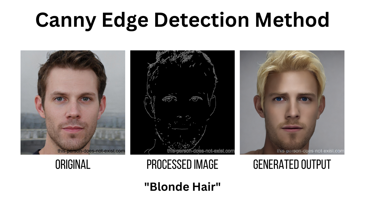
Canny edge detection is a method that uses a special algorithm to detect edges in images that are further used by the model to edit the image. In this section, implement the Canny Edge Detection method in ControlNet as described in the steps below.

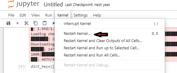
1. To clear GPU memory and start running the model, navigate to the Kernel menu option in your Jupyter Notebook, and click Restart Kernel.

   

2. Import the required libraries you installed earlier

3. Import the additional libraries required by the model

    import cv2
    import numpy as np

   Below is what the additional libraries do:

   • cv2: Provides all the functions and capabilities provided by OpenCV. These include reading and writing images, image manipulation, image processing techniques like edge detection, feature detection and matching
   • numpy: It's used for numerical computing. Together, cv2 and numpy enable efficient and flexible image processing

4. Import the base image to the image variable

    image = load_image("https://example.com/image.png")

   To use apply the image to the model, verify that your URL has a valid file extension such as .png, .jpg, or jpeg

5. Convert the image into a NumPy array

    image = np.array(image)

   Many Computer Vision (CV) tasks run in NumPy format due to their efficiency and ease of manipulation. The above command converts a Python Imaging Library (PIL) image to a NumPy array.

6. Define thresholds

    low_threshold = 100
    high_threshold = 200

   low_threshold and high_threshold define the sensitivity and robustness of the edge detection process. low_threshold allows detection of weaker edges, but leads to more noise in the classification. A larger high_threshold value results in the detection of less strong edges potentially missing some edges.

7. Process the image

    image = cv2.Canny(image, low_threshold, high_threshold)
    image = image[:, :, None]
    image = np.concatenate([image, image, image], axis=2)
    image = Image.fromarray(image)

   Below is the processing performed by the above code:

   • cv2.Canny(image, low_threshold, high_threshold): Applies the Canny edge detection to the image NumPy array using the cv2.Canny() function
   • image[:, :, None]: Adds a new axis to the NumPy array image, converting it from a 2D grayscale image to a 3D image with a single channel because the Canny function generates a binary image
   • np.concatenate([image, image, image], axis=2): Concatenates the image array along the third axis to create a 3-channel image. This is necessary because most image processing operations require images with three channels (RGB), but the Canny edge detection only produces a single-channel image.
   • Image.fromarray(image): Converts the NumPy array image back into a PIL image to save, display, or perform other PIL operations on the image.

8. Define the model.

    controlnet = ControlNetModel.from_pretrained(
    "lllyasviel/sd-controlnet-canny"
    )
    pipe = StableDiffusionControlNetPipeline.from_pretrained(
       "runwayml/stable-diffusion-v1-5", controlnet=controlnet, safety_checker=None
    )
    pipe.scheduler = UniPCMultistepScheduler.from_config(pipe.scheduler.config)
    pipe.enable_model_cpu_offload()

   In the above code:

   • controlnet: Initializes the ControlNetModel model using a pre-trained dataset from lllyasviel/sd-controlnet-canny
   • pipe: Initializes the StableDiffusionControlNetPipeline pipeline for stable diffusion-based image processing. It utilizes the previously created ControlNet model for controlling the diffusion process. The safety checker parameter, when set to None results in no safety checks in the pipeline
   • pipe.scheduler: Initializes the UniPCMultistepScheduler scheduler to control and schedule the execution of the diffusion process in a stable manner
   • enable_model_cpu_offload(): Enables CPU offloading for the model used in the ControlNetModel pipeline. It refers to the practice of running parts of a computational workload on the CPU instead of the GPU.

9. Using a prompt, execute the defined model on the image

    image = pipe("YOUR_TEXT_PROMPT_HERE", image, num_inference_steps=20).images[0]

   To apply a prompt such as, "make their hair blond", or "make their shirt green", edit your prompt like below

    image = pipe("make their hair blond", image, num_inference_steps=20).images[0]

   The above code executes the StableDiffusionControlNetPipeline on the input image. The text prompt defines the changes required in the image. The num_inference_steps parameter specifies the number of diffusion steps the pipeline should perform. It's set to 20 but it's reduced or increased depending on how much of the original image you want to keep.

10. View the generated image

     image

Depth Map Method

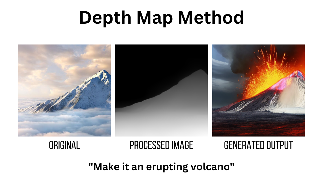
The ControlNet depth map method provides spatial information about the image, indicating the depth or distance of different parts of the scene from the camera's perspective, and helps to create a non-RGB 3D image for further processing.

1. To run the model, restart your Jupyter Notebook kernel

   

2. Import the required libraries you installed earlier

3. Import the additional libraries for this model

    from transformers import pipeline
    import numpy as np

   In the above code, transformers provides a wide range of Natural Language Processing (NLP) models for tasks such as text classification. The pipeline function is a transformers library API that uses pre-trained models for specific NLP tasks

4. Define the pipeline that takes in a task argument which is depth-estimation

    depth_estimator = pipeline('depth-estimation')

5. Load the image

    image = load_image("https://example.com/image.png")

6. Retrieve the Depth Map and convert the image into a NumPy array.

    image = depth_estimator(image)['depth']
    image = np.array(image)

7. Process the image

    image = image[:, :, None]
    image = np.concatenate([image, image, image], axis=2)
    image = Image.fromarray(image)

8. Define the model

    controlnet = ControlNetModel.from_pretrained(
    "lllyasviel/sd-controlnet-depth"
    )
    pipe = StableDiffusionControlNetPipeline.from_pretrained(
        "runwayml/stable-diffusion-v1-5", controlnet=controlnet, safety_checker=None
    )
    pipe.scheduler = UniPCMultistepScheduler.from_config(pipe.scheduler.config)
    pipe.enable_model_cpu_offload()

9. Execute the model on the image with a text prompt

    image = pipe("YOUR_TEXT_PROMPT_HERE", image, num_inference_steps=20).images[0]

10. View the generated image

    image

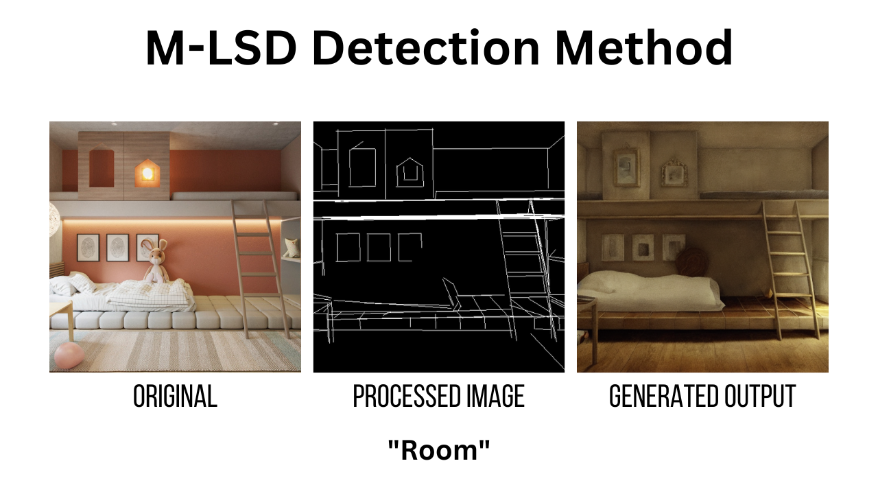
M-LSD Detection Method

M-LSD is an algorithm used to detect the outline of an image which includes the line segments. In this section, use the M-LSD detection with ControlNet as described below.

1. Restart your Jupyter Notebook kernel to clear GPU memory

   

2. Import the required libraries

3. Import the additional library for this model

    from controlnet_aux import MLSDdetector
    import matplotlib

4. Initialize the model with a pre-trained model

    mlsd = MLSDdetector.from_pretrained('lllyasviel/ControlNet')

5. Import the image and apply the MLSDdetector

    image = load_image("https://example.com/image.png")
    image = mlsd(image)

6. Define the model

    controlnet = ControlNetModel.from_pretrained(
    "lllyasviel/sd-controlnet-mlsd"
    )
    pipe = StableDiffusionControlNetPipeline.from_pretrained(
        "runwayml/stable-diffusion-v1-5", controlnet=controlnet, safety_checker=None
    )
    pipe.scheduler = UniPCMultistepScheduler.from_config(pipe.scheduler.config)
    pipe.enable_model_cpu_offload()

7. Execute the model on the image with prompt

    image = pipe("YOUR_TEXT_PROMPT_HERE", image, num_inference_steps=20).images[0]

8. View the generated image

    image

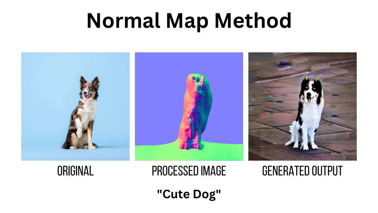
Normal Map Method

In a normal map, pixels encode in the direction of the surface normal in RGB. By encoding the surface normal as color information, the normal map provides a way of storing and representing detailed surface information without increasing the model complexity.

1. To run the model, restart your Jupyter Notebook kernel

   

2. Import the required libraries

3. Import the additional libraries required for this model.

    from transformers import pipeline
    import numpy as np
    import cv2

4. Import the base image

    image = load_image("https://example.com/image.png").convert("RGB")

   When the image imports to the image variable, it's converted into the standard color representation RGB.

5. Import the model and assign the image to the model

    depth_estimator = pipeline("depth-estimation", model="Intel/dpt-hybrid-midas" )
    image = depth_estimator(image)['predicted_depth'][0]

6. Convert the image into a NumPy array

    image = image.numpy()

7. Process the image

    image_depth = image.copy()
    image_depth -= np.min(image_depth)
    image_depth /= np.max(image_depth)
    bg_threhold = 0.4
    x = cv2.Sobel(image, cv2.CV_32F, 1, 0, ksize=3)
    x[image_depth < bg_threhold] = 0
    y = cv2.Sobel(image, cv2.CV_32F, 0, 1, ksize=3)
    y[image_depth < bg_threhold] = 0
    z = np.ones_like(x) * np.pi * 2.0
    image = np.stack([x, y, z], axis=2)
    image /= np.sum(image ** 2.0, axis=2, keepdims=True) ** 0.5
    image = (image * 127.5 + 127.5).clip(0, 255).astype(np.uint8)
    image = Image.fromarray(image)

   Below is what the code does:

   • image_depth: Stores a copy of the image from the NumPy array
   • image_depth -= np.min(image_depth): Subtracts the minimum pixel value from the image_depth array and normalizes it to ensure all pixel values are non-negative
   • image_depth /= np.max(image_depth): Scales the pixel values to the range [0, 1] by dividing the entire image_depth array with its maximum value
   • bg_threhold = 0.4: Defines a threshold value (0.4 in this case) to identify the background pixels in the depth map. Pixels with a value less than the threshold are background pixels
   • x = cv2.Sobel(image, cv2.CV_32F, 1, 0, ksize=3): Applies the Sobel operator on the original image along the x-axis to compute the gradient in the x-direction. The resulting x array represents the x-component
   • x[image_depth < bg_threhold] = 0: Removes the gradients from the background regions. The same processes run for the y-direction
   • z = np.ones_like(x) * np.pi * 2.0: Initializes an array z with the same shape as x and fills it with a constant value of 2.0 * np.pi. The z component represents the orientation angle of the gradient
   • np.stack([x, y, z], axis=2): The x, y, and z arrays combine along the third dimension to create a 3-channel image
   • np.sum(image ** 2.0, axis=2, keepdims=True) ** 0.5: Normalizes the combined gradient image to unit length. It divides each pixel's gradient vector by its value, ensuring that the gradient vectors have a length of 1
   • (image * 127.5 + 127.5).clip(0, 255).astype(np.uint8): Ensures that the gradient image scales and shifts to the range [0, 255] for visualization as an 8-bit image
   • image = Image.fromarray(image): Converts the NumPy array image to an Image object from PIL for visualization or other uses

8. Define the model

    controlnet = ControlNetModel.from_pretrained(
    "fusing/stable-diffusion-v1-5-controlnet-normal"
    )
    pipe = StableDiffusionControlNetPipeline.from_pretrained(
        "runwayml/stable-diffusion-v1-5", controlnet=controlnet, safety_checker=None
    )
    pipe.scheduler = UniPCMultistepScheduler.from_config(pipe.scheduler.config)
    pipe.enable_model_cpu_offload()

9. Execute the model on the image with a text prompt

    image = pipe("YOUR_PROMPT_HERE", image, num_inference_steps=20).images[0]

10. View the image

    image

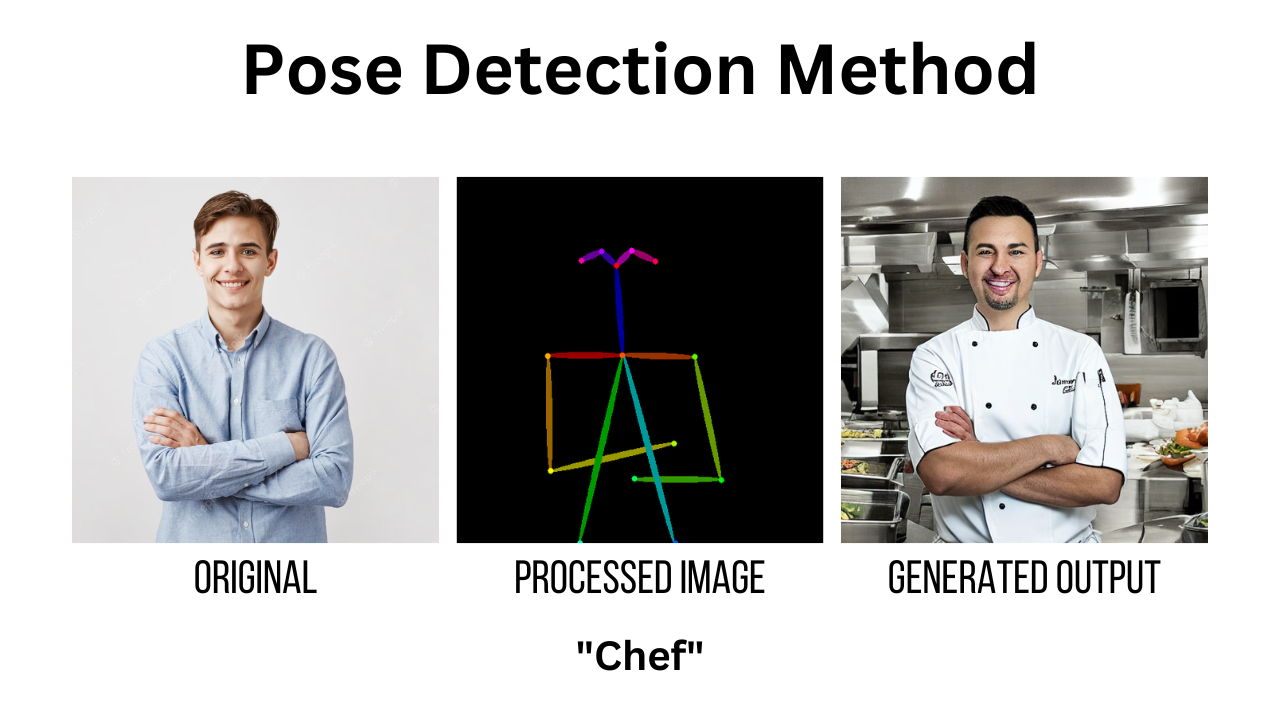
Pose Detection Method

This model detects the pose from an image and makes changes based on the retrieved pose information. The pose is always retained in this model irrespective of the required changes as described below.

1. Restart the Jupyter Notebook kernel to run the model

   

2. Import the required libraries

3. Import the openpose detector used to detect the pose in an image

    from controlnet_aux import OpenposeDetector

4. Initialize the model with the pre-trained model and store it in a variable

    openpose = OpenposeDetector.from_pretrained('lllyasviel/ControlNet')

   The OpenposeDetector performs pose estimation, a computer vision task that involves detecting and localizing human body key points in an image. It's initialized with a pre-trained model for faster execution.

5. Load the image and pass it to the initialized openpose variable

    image = load_image("https://example.com/image.png")
    image = openpose(image)

6. Define the model

    controlnet = ControlNetModel.from_pretrained(
        "lllyasviel/sd-controlnet-openpose"
    )
    pipe = StableDiffusionControlNetPipeline.from_pretrained(
        "runwayml/stable-diffusion-v1-5", controlnet=controlnet, safety_checker=None
    )
    pipe.scheduler = UniPCMultistepScheduler.from_config(pipe.scheduler.config)
    pipe.enable_model_cpu_offload()

7. Using a prompt, execute the model on the image

    image = pipe("YOUR_PROMPT_HERE", image, num_inference_steps=20).images[0]

8. View the generated image

    image

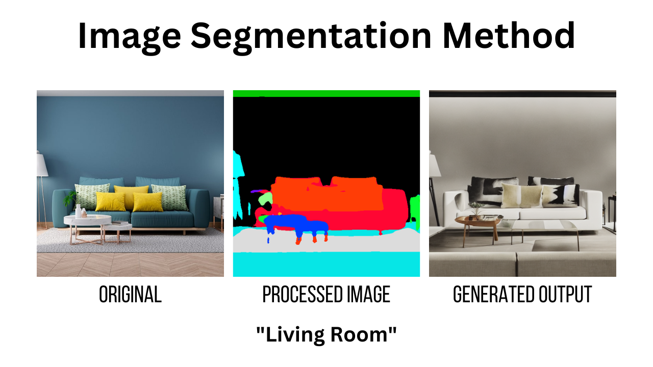
Image Segmentation Method

Image segmentation is a method in which image processing uses the partition of an image into multiple parts or regions, based on the characteristics of the image pixels. Apply the image segmentation ControlNet method as described in the steps below.

1. Restart your Jupyter Notebook kernel

   

2. Import the required libraries

3. Import the additional libraries required for this model

    from transformers import AutoImageProcessor, UperNetForSemanticSegmentation
    import numpy as np

4. Using numpy, define a color palette

    palette = np.asarray([ [0, 0, 0], [120, 120, 120], [180, 120, 120], [6, 230, 230], [80, 50, 50], [4, 200, 3], [120, 120, 80], [140, 140, 140], [204, 5, 255], [230, 230, 230], [4, 250, 7], [224, 5, 255], [235, 255, 7], [150, 5, 61], [120, 120, 70], [8, 255, 51], [255, 6, 82], [143, 255, 140], [204, 255, 4], [255, 51, 7], [204, 70, 3], [0, 102, 200], [61, 230, 250], [255, 6, 51], [11, 102, 255], [255, 7, 71], [255, 9, 224], [9, 7, 230], [220, 220, 220], [255, 9, 92], [112, 9, 255], [8, 255, 214], [7, 255, 224], [255, 184, 6], [10, 255, 71], [255, 41, 10], [7, 255, 255], [224, 255, 8], [102, 8, 255], [255, 61, 6], [255, 194, 7], [255, 122, 8], [0, 255, 20], [255, 8, 41], [255, 5, 153], [6, 51, 255], [235, 12, 255], [160, 150, 20], [0, 163, 255], [140, 140, 140], [250, 10, 15], [20, 255, 0], [31, 255, 0], [255, 31, 0], [255, 224, 0], [153, 255, 0], [0, 0, 255], [255, 71, 0], [0, 235, 255], [0, 173, 255], [31, 0, 255], [11, 200, 200], [255, 82, 0], [0, 255, 245], [0, 61, 255], [0, 255, 112], [0, 255, 133], [255, 0, 0], [255, 163, 0], [255, 102, 0], [194, 255, 0], [0, 143, 255], [51, 255, 0], [0, 82, 255], [0, 255, 41], [0, 255, 173], [10, 0, 255], [173, 255, 0], [0, 255, 153], [255, 92, 0], [255, 0, 255], [255, 0, 245], [255, 0, 102], [255, 173, 0], [255, 0, 20], [255, 184, 184], [0, 31, 255], [0, 255, 61], [0, 71, 255], [255, 0, 204], [0, 255, 194], [0, 255, 82], [0, 10, 255], [0, 112, 255], [51, 0, 255], [0, 194, 255], [0, 122, 255], [0, 255, 163], [255, 153, 0], [0, 255, 10], [255, 112, 0], [143, 255, 0], [82, 0, 255], [163, 255, 0], [255, 235, 0], [8, 184, 170], [133, 0, 255], [0, 255, 92], [184, 0, 255], [255, 0, 31], [0, 184, 255], [0, 214, 255], [255, 0, 112], [92, 255, 0], [0, 224, 255], [112, 224, 255], [70, 184, 160], [163, 0, 255], [153, 0, 255], [71, 255, 0], [255, 0, 163], [255, 204, 0], [255, 0, 143], [0, 255, 235], [133, 255, 0], [255, 0, 235], [245, 0, 255], [255, 0, 122], [255, 245, 0], [10, 190, 212], [214, 255, 0], [0, 204, 255], [20, 0, 255], [255, 255, 0], [0, 153, 255], [0, 41, 255], [0, 255, 204], [41, 0, 255], [41, 255, 0], [173, 0, 255], [0, 245, 255], [71, 0, 255], [122, 0, 255], [0, 255, 184], [0, 92, 255], [184, 255, 0], [0, 133, 255], [255, 214, 0], [25, 194, 194], [102, 255, 0], [92, 0, 255], ])

5. Define the image processor and segmentor

    image_processor = AutoImageProcessor.from_pretrained("openmmlab/upernet-convnext-small")
    image_segmentor = UperNetForSemanticSegmentation.from_pretrained("openmmlab/upernet-convnext-small")

   In the above code:

   • AutoImageProcessor: Handles different image processing tasks such as resizing, normalization, and padding. The upernet-convnext-small model is a lighter version of UperNet, which is a semantic segmentation model.
   • UperNetForSemanticSegmentation: This function is a class designed for semantic segmentation tasks using the UperNet architecture. The upernet-convnext-small model trains on a large dataset that segments images into different classes to represent objects or regions with the same semantic meaning.

   Both of the functions run on a pre-trained model to perform semantic segmentation on input images

6. Load the Image and convert it to RGB

    image = load_image("https://example.com/image.png").convert('RGB')

7. Process the image

    pixel_values = image_processor(image, return_tensors="pt").pixel_values
    with torch.no_grad():
      outputs = image_segmentor(pixel_values)
    seg = image_processor.post_process_semantic_segmentation(outputs, target_sizes=[image.size[::-1]])[0]
    color_seg = np.zeros((seg.shape[0], seg.shape[1], 3), dtype=np.uint8) # height, width, 3
    for label, color in enumerate(palette):
        color_seg[seg == label, :] = color
    color_seg = color_seg.astype(np.uint8)
    image = Image.fromarray(color_seg)

   The above code defines the functions below:

   • image_processor: Pre-processes the input image. It takes the image as an argument and returns the image as a PyTorch tensor. The return_tensors="pt" argument sets the output to a PyTorch tensor
   • torch.no_grad(): Temporarily disables the gradient computation
   • pixel_values: Passes the processed image through image_processor, and obtains pixel values of the processed image
   • image_segmentor: Takes the processed image as input and produces segmentation outputs
   • seg: Passes the image_processor.post_process_semantic_segmentation function. It takes the model outputs and the target size of the image [image.size[::-1]] as an argument to return the segmented image
   • color_seg: An empty numpy array that stores the dimensions of the input image
   • for label, color in enumerate(palette): Iterates over each label and its corresponding color in the palette
   • color_seg[seg == label, :] = color: Assigns the corresponding color to each pixel in color_seg based on the class label from the segmentation seg
   • color_seg.astype(np.uint8): Converts a segmented image to a numpy array with unsigned 8-bit integers
   • Image.fromarray(color_seg): Converts the numpy array color_seg to an Image object from PIL

8. Define the model

    controlnet = ControlNetModel.from_pretrained(
        "lllyasviel/sd-controlnet-seg"
    )
    pipe = StableDiffusionControlNetPipeline.from_pretrained(
        "runwayml/stable-diffusion-v1-5", controlnet=controlnet, safety_checker=None
    )
    pipe.scheduler = UniPCMultistepScheduler.from_config(pipe.scheduler.config)
    pipe.enable_model_cpu_offload()

9. Execute the model on the image with a text prompt

    image = pipe("YOUR_PROMPT_HERE", image, num_inference_steps=20).images[0]

10. View the generated image

     image

Additional Model Parameters

Each model supports additional parameters that allow you to fine-tune the output, save the generated image, and change the precision mode as described in the optional steps below.

1. To save the generated image, view your working directory

    pwd

2. Save your Image to the working directory path. For example, in your user home directory

    image.save("/home/user/")

   To save the image to a different path. Create the target directory first, and set it as the output path. For example, when you create a model-images directory, use:

    image.save("/home/user/model-images")

3. To view the processed image before the model executes. Run the image variable to view its value

    image

   When you run the following prompt, the model executes on the variable, and when run again, you instead view the final generated output.

    image = pipe("YOUR_PROMPT_HERE", image, num_inference_steps=20).images[0]

4. To view the final generated output, run the variable after the model executes the image as below

    image = pipe("YOUR_PROMPT_HERE", image, num_inference_steps=20).images[0]
    image

   In summary, running the variable before the prompt returns the processed image while running it after returns the final generated output.

5. To run the model on half-bit precision for faster execution, apply the torch_dtype as torch.float16 to the pipeline as below

    controlnet = ControlNetModel.from_pretrained(
    "THE_MODEL_NAME_HERE",torch_dtype=torch.float16
    )
    pipe = StableDiffusionControlNetPipeline.from_pretrained(
       "runwayml/stable-diffusion-v1-5", controlnet=controlnet, safety_checker=None,torch_dtype=torch.float16
    )

   It's important to note that using half-bit precision makes the model less precise

6. To optimize the model for faster speed and reduced memory consumption, use xformers before running executing the model on the image

    pipe.enable_xformers_memory_efficient_attention()

Conclusion

In this article, you implemented Image manipulation with Stable Diffusion ControlNet models on a Vultr Cloud GPU server. You set up the server, installed common libraries, and performed image processing using the available model methods.

More Information

For more information about ControlNet methods, visit the following model card pages.

• Model Card for Canny Edge Detection Method
• Model Card for Depth Map Method
• Model Card for M-LSD Detection Method
• Model Card for Normal Map Method
• Model Card for Pose Detection Method
• Model Card for Image Segmentation Method