

Neural Style Transfer involves styling an image using an artificial system based on a Deep Neural Network. In the styling process, algorithms manipulate the content image to generate a new image with the artistic style of another image.
Developed by Leon A. Gatys, Alexander S. Ecker, and Matthias Bethge, the practical application of machine learning was seen in 2015. As per the research paper "A Neural Algorithm of Artistic Style" by Leon A. Gatys, the content and style of the images are separated and recombined using neural representations to generate artistic results through a neural algorithm.
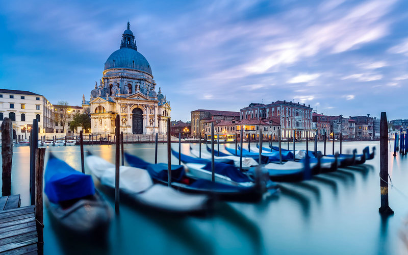
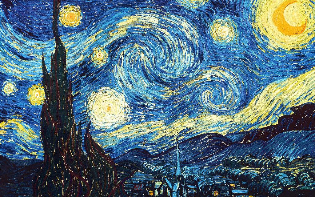
The optimization technique uses two images -- content image and style reference image. The style reference image is any artistic image designed by a painter. The images are optimized to match the content and style statistics from the content and the style reference image extracted using a convolutional network. The optimized output image generated resembles the content image, but it imprints the style of the reference image.
In the tutorial, we will understand the VGG-19 neural styling method and perform the neural style transfer on user images using Python3 and PyTorch on the Windows operating system.
1. The VGG-19 Styling Process
In this tutorial, you need a pre-trained network and VGG-19 network to perform Neural Style Transfer (NST). Here you will freeze the VGG-19 network so that weights in the network remain constant.
VGG-19 is an image recognition technology that pushes the images to a depth of 19 layers.
The NST process uses three images: the content image and the style reference image as inputs, and the generated image as output. Through the training process, the output image generated resembles the content image blended with the style of the reference image.
Each of the three images go through the VGG network separately. While extracting the output image, you need only specified convoluted layers. According to the research paper, there are five convoluted layers. These are conv 1-1, conv 2-1, conv 3-1, conv 4-1, and conv 5-1, where the first digit changes after the image layer goes through a maxpool layer.
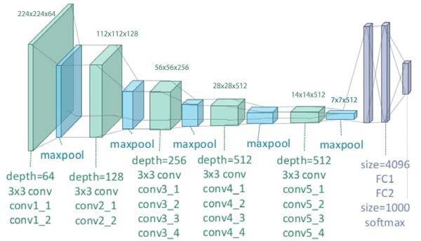
Since NST uses three images, the VGG network will have a 3x output of five convoluted layers. You need to optimize the layers through a loss function having three components: total loss, content loss, and style loss.
- The total variation loss is a linear combination between the content loss and the style loss. It is represented by a hyperparameter alpha times content loss and beta times style loss.

- The content loss compares the features of the content image and generated image by taking the norm for every layer.

In the above equation, a = output of one of the five convolutional layers l = denotes the number of convolutional layers from where you will extract the output C= content image G= generated image
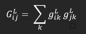
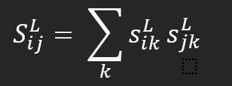
- It isn't easy to capture style loss as deep learning comes into play. You need to frame the Gram matrices for the generated and the style image. Essentially in the Gram matrices, the output is multiplied with its transpose.
2. Requirements and Dependencies
2.1 Pre-requisites
To proceed with the tutorial, you need a computer system with the following installed:
conda package and environment management system. It creates a virtual python environment pre-loaded with all the necessary packages and their dependencies. The latest version of the anaconda distribution comes with Python 3.9.13, essential for installing PyTorch libraries.
PyTorch The python based computing package is only compatible with specific versions of Python 3. The conda package manager is pre-loaded with Python 3.9, which enables seamless installation of PyTorch and its libraries. Follow the official docs of PyTorch to install the library through the conda package system.
Code editors Visual Studio Code or Jupyter Notebook for running the NST code.
2.2 Importing packages
After you install the PyTorch library using the conda environment, use code editors like Jupyter Notebook or VS Code to complete the tutorial.
torchandtorch.nnthese are indispensable packages for using neural networks in PyTorchtorch.optimdenotes the efficient gradient descentsPILis used to load and display imagestorchvision.transformsit converts PIL images into tensorstorchvision.modelstrains or loads the pre-trained VGG-19 modeltorchvision.utilsstores the generated image after the transfer is completeimport torch import torch.nn as nn import torch.optim as optim from PIL import Image import torchvision.transforms as transforms import torchvision.models as models from torchvision.utils import save_image
3. How to run an experiment on neural style transfer using Jupyter Notebook?
Install all the packages, then display the convolution layers. To get all the convolution layers, use the command models.vgg19
model = models.vgg19(weights=True).featuresTo check the convolution layers, print the variable:
print(model)Concerning the VGG-19 architecture, the following output denotes all the convoluted layers after going through the VGG network separately. Figure out the layers denoting conv1-1, conv2-1, conv3-1, conv4-1, and conv5-1 extracted after maxpool. Thus, take the layers at 0, 5, 10, 19, and 28, which correspond to conv1-1, conv2-1, conv3-1, conv4-1, and conv5-1.
But what about the layers after 28? Those layers are unnecessary as they carry no value in the loss function.
Sequential(
    (0): Conv2d(3, 64, kernel_size=(3, 3), stride=(1, 1), padding=(1, 1))
    (1): ReLU(inplace=True)
    (2): Conv2d(64, 64, kernel_size=(3, 3), stride=(1, 1), padding=(1, 1))
    (3): ReLU(inplace=True)
    (4): MaxPool2d(kernel_size=2, stride=2, padding=0, dilation=1, ceil_mode=False)
    (5): Conv2d(64, 128, kernel_size=(3, 3), stride=(1, 1), padding=(1, 1))
    (6): ReLU(inplace=True)
    (7): Conv2d(128, 128, kernel_size=(3, 3), stride=(1, 1), padding=(1, 1))
    (8): ReLU(inplace=True)
    (9): MaxPool2d(kernel_size=2, stride=2, padding=0, dilation=1, ceil_mode=False)
    (10): Conv2d(128, 256, kernel_size=(3, 3), stride=(1, 1), padding=(1, 1))
    (11): ReLU(inplace=True)
    (12): Conv2d(256, 256, kernel_size=(3, 3), stride=(1, 1), padding=(1, 1))
    (13): ReLU(inplace=True)
    (14): Conv2d(256, 256, kernel_size=(3, 3), stride=(1, 1), padding=(1, 1))
    (15): ReLU(inplace=True)
    (16): Conv2d(256, 256, kernel_size=(3, 3), stride=(1, 1), padding=(1, 1))
    (17): ReLU(inplace=True)
    (18): MaxPool2d(kernel_size=2, stride=2, padding=0, dilation=1, ceil_mode=False)
    (19): Conv2d(256, 512, kernel_size=(3, 3), stride=(1, 1), padding=(1, 1))
    (20): ReLU(inplace=True)
    (21): Conv2d(512, 512, kernel_size=(3, 3), stride=(1, 1), padding=(1, 1))
    (22): ReLU(inplace=True)
    (23): Conv2d(512, 512, kernel_size=(3, 3), stride=(1, 1), padding=(1, 1))
    (24): ReLU(inplace=True)
    (25): Conv2d(512, 512, kernel_size=(3, 3), stride=(1, 1), padding=(1, 1))
    (26): ReLU(inplace=True)
    (27): MaxPool2d(kernel_size=2, stride=2, padding=0, dilation=1, ceil_mode=False)
    (28): Conv2d(512, 512, kernel_size=(3, 3), stride=(1, 1), padding=(1, 1))
    (29): ReLU(inplace=True)
    (30): Conv2d(512, 512, kernel_size=(3, 3), stride=(1, 1), padding=(1, 1))
    (31): ReLU(inplace=True)
    (32): Conv2d(512, 512, kernel_size=(3, 3), stride=(1, 1), padding=(1, 1))
    (33): ReLU(inplace=True)
    (34): Conv2d(512, 512, kernel_size=(3, 3), stride=(1, 1), padding=(1, 1))
    (35): ReLU(inplace=True)
    (36): MaxPool2d(kernel_size=2, stride=2, padding=0, dilation=1, ceil_mode=False)
    )
4. Transforming user images using PyTorch and Python3
4.1 Setting the training loop
Now you know which conv layers to extract to proceed with the tutorial.
Create a class VGG'and inherit from the nn.Module`
Define function _init_ of self and call an overridden method VGG, self-using super
Now use the chosen features ['0', '5', '10', '19', '28'] representing the extracted output upon completing the neural style transfer.
Complete the function by generating the model up to the 28th feature and excluding the rest.
class VGG(nn.Module):
def __init__(self):
    super(VGG,self).__init__()

    self.chosen_features = ['0', '5', '10', '19', '28']
    self.model = models.vgg19(weights=True).features[:29]
Define another function called forward with parameters self, x.
Store all the features upon generation so define an empty array or a list.
For all the layers in the self.model, send x through those layers, and then call the output using x.
If the layer_num is in the chosen_features list, then append it to the empty array.
Complete the function by returning the feature.
def forward(self,x):
    features =[]

    for layer_num, layer in enumerate(self.model):
        x = layer(x)

        if str(layer_num) in self.chosen_features:
            features.append(x)

    return feature
The device or the loader is not yet defined. Select a device to import the content and style images and run the VGG-19 network. Usually, running the neural style transfer algorithm takes a long time on large images. But a GPU speeds up the process. Use torch.cuda.is_available() to check if a GPU is available in the system. After you determine the device, set torch.device to use the same device throughout.
.to(device) method is used to move tensors or modules to a desired device.
To specify the image_size, for a CPU, use a lower number like 356, which would be a decent size. Else train the algorithm on a larger image using a graphics card. But it takes a longer time.
While using the content and style reference images, ensure that the size is the same. If it is not the same, you cannot subtract them while calculating the loss.
transforms.ToTensor converts both the images into tensors.
device = torch.device("cuda" if torch.cuda.is_available else "cpu"
    #device = torch.device("cpu")
    image_size =500
4.2 Loading the images
Import the content and the style images. Initially, the value of PIL images lies between 0 and 255. After you transform it into torch tensors, it converts and lies within the range of 0 to 1.
Resize the images to match their dimensions. Take note that the training of the neural networks from the PyTorch library is completed only with tensor values from 0 to 1. In case you feed the networks with tensor images lying between 0 to 255, then content and style goes undetected by the activated feature maps.
To load the image, define a function load_image and use a parameter image_name.
Initialize an image variable to Image. Here is where the PIL library comes into play.
Load the image using the loader
unsqueeze(0) is used to add dimension for the batch size.
While using the content and the style reference image, place both in the same folder. Load them in the program.
The output-generated image can be present as noise. In this case, let us replicate the content image. You can create a copy of the original image using original_img.clone(). making it faster than using noise.
reguires_grad_(True) is essential as you need to freeze the network. The only thing that can change is the generated image.
loader = transforms.Compose(
[
    transforms.Resize((image_size, image_size)), # scale imported images
    transforms.ToTensor(), # transform it into a torch tensor
]
)

    def load_image(image_name):
        image = Image.open(image_name)
        image = loader(image).unsqueeze(0)
        return image.to(device)

    original_img = load_image("content_image.jpg")
    style_img = load_image("style_image.jpg")

    model = VGG().to(device).eval()
    generated = original_img.clone().requires_grad_(True)
4.3 Setting the hyperparameters
You need to select the hyperparameters.
total_steps , learning_rate , alpha , and beta
    total_steps = 6000
    learning_rate = 0.001
    alpha = 1
    beta = 0.01
    optimizer = optim.Adam([generated], lr= learning_rate)
Run a for loop to determine the number of times the image modifies.
Send each of the three images through the VGG-19 network.
While running through a list of output from five different conv layers, find the style loss and the content loss beforehand by initializing them to 0.
for step in range(total_steps):
generated_features = model(generated)
original_img_features = model(original_img)
style_features = model(style_img)
style_loss = original_loss = 0
4.4 Calculating the Loss Function
Iterate through all of the features for the chosen layers. Run a for loop for the aspects in the three images from the conv layers. Consider conv1_1 for the generated image, the content image, and the style reference image. But nevertheless, you have to iterate through all five layers.
Calculate the content loss with the torch.mean, which returns the mean of all the values after subtracting the original features from the generated aspects in the input tensor.
Compute the gram matrices for the generated and the style image according to the theory mentioned in section 1. Multiply the pixel value of each channel by other channels for the new features generated. Concluding with shape channel by channel, the generated gram matrix is subtracted from the style gram matrix. The gram matrix calculates a kind of correlation matrix. If the pixel colors are similar across the channels of the generated image and the style image, then that results in the two pictures having a similar style.
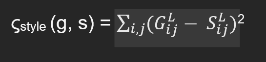
Calculate the style loss and the total loss when you have the gram matrices for both generated and style images.
With total loss perform total_loss.backward() and optimizer.step()
for gen_feature, orig_feature, style_features in zip(
    generated_features, original_img_features, style_features):

    batch_size, channel, height, width = gen_feature.shape
    original_loss += torch.mean((gen_feature - orig_feature) **2 )


    G = gen_feature.view(channel, height*width).mm(
        gen_feature.view(channel, height*width).t()
    )

    A = style_features.view(channel, height*width).mm(
        style_features.view(channel, height*width).t()
    )

    style_loss +=torch.mean((G - A)**2)

total_loss = alpha*original_loss + beta * style_loss
optimizer.zero_grad()
total_loss.backward()
optimizer.step()
Complete the program by printing the total loss that the algorithm concurs with and saving the generated image.
 if step % 200 == 0:
    print(total_loss)
    save_image(generated, "generated_image.png")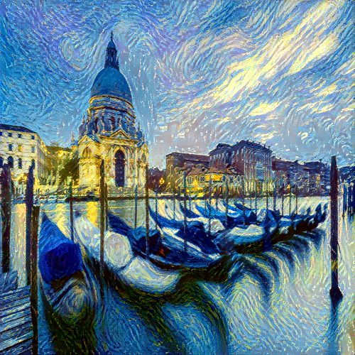
4.5 Output
The output console displays the total loss after every 200 steps. The more you train the model and play with the hyperparameters, the better the generated image.
tensor(5365698., grad_fn=<AddBackward0>)
    tensor(100573.4922, grad_fn=<AddBackward0>)
    tensor(40841.7070, grad_fn=<AddBackward0>)
    tensor(23182.7207, grad_fn=<AddBackward0>)
    tensor(15629.9502, grad_fn=<AddBackward0>)
    tensor(11835.2373, grad_fn=<AddBackward0>)
    tensor(9588.9961, grad_fn=<AddBackward0>)
    tensor(8060.4053, grad_fn=<AddBackward0>)
    tensor(6925.2471, grad_fn=<AddBackward0>)
    tensor(6039.4619, grad_fn=<AddBackward0>)
    tensor(5327.7583, grad_fn=<AddBackward0>)
    tensor(4743.5991, grad_fn=<AddBackward0>)
    tensor(4255.8604, grad_fn=<AddBackward0>)
    tensor(3845.0798, grad_fn=<AddBackward0>)
    tensor(3493.4805, grad_fn=<AddBackward0>)
    tensor(3190.8813, grad_fn=<AddBackward0>)
    tensor(2926.9409, grad_fn=<AddBackward0>)
    tensor(2694.3345, grad_fn=<AddBackward0>)
    tensor(2488.2522, grad_fn=<AddBackward0>)
    tensor(2304.4019, grad_fn=<AddBackward0>)
    tensor(2139.8572, grad_fn=<AddBackward0>)
    tensor(1991.9841, grad_fn=<AddBackward0>)
    tensor(1858.3828, grad_fn=<AddBackward0>)
    tensor(1737.2626, grad_fn=<AddBackward0>)
    tensor(1627.4678, grad_fn=<AddBackward0>)
    tensor(1527.8431, grad_fn=<AddBackward0>)
    tensor(1436.7794, grad_fn=<AddBackward0>)
    tensor(1352.9731, grad_fn=<AddBackward0>)
    tensor(1275.8182, grad_fn=<AddBackward0>)
    tensor(1204.6921, grad_fn=<AddBackward0>)
Conclusion and Key Takeaways
In this tutorial, you implemented neural style transfer on the Windows OS. The step-by-step guide utilized Python3 and PyTorch to transfer the style of the reference image to the original image. NST is a process that utilizes Deep Neural Network to generate images with different artistic styles. The tutorial covered the VGG-19 neural styling process, in which you used three images and five convolution layers.
Machine learning and AI have diverse applications, and neural style transfer is one of them. Vultur has a good collection of technical documents which are worth exploring:
- Here is a list of articles published by various authors across diverse technologies.
- Try building a Machine Learning classifier using Python and Scikit Learn.
- Learn about the open source deep learning model called stable diffusion and generate images using a text prompt.
No comments yet.